Computer Vision Tasks

There are several core tasks in Computer Vision:

Classification: assign one label to the whole image
Semantic Segmentation: assign one semantic class to each pixel
Object Detection: find objects and output bounding boxes + class labels
Instance Segmentation: do detection and also output a mask for each object instance

A useful distinction:

classification has no spatial extent
semantic segmentation cares about all pixels
object detection cares about multiple objects and their boxes
instance segmentation cares about multiple objects and their masks

Semantic Segmentation

The problem

In semantic segmentation, we want to classify every pixel in an image.

Training data:

input image
target segmentation mask
each pixel in the mask is labeled by a semantic category such as grass, sky, cat, tree, road, etc.

At test time:

input a new image
predict one semantic class per pixel

Sliding window

A very early idea is:

take a patch around one pixel
run a CNN on the patch
classify the center pixel

This gives local context, which is important because:

a single pixel alone is often ambiguous
surrounding pixels help identify the object / region

But this approach has an obvious problem:

Problem:

very inefficient
overlapping patches share most of their pixels
the network repeatedly recomputes almost the same features

Fully convolutional idea

A much better idea is to process the whole image at once.

High-level idea: use a network made of convolutional layers so that we predict pixel labels for all positions in parallel.

If the network outputs class scores for each pixel, then:

input shape: $3 \times H \times W$
output score map: $C \times H \times W$
final prediction: take argmax over the class dimension

This is the idea behind Fully Convolutional Networks (FCN).

The difficulty: resolution

Classification networks usually:

use pooling / stride
reduce spatial resolution
go deeper with lower-resolution features

But segmentation requires:

output resolution to match the input resolution
fine spatial boundaries

So the network must contain both:

downsampling to get larger receptive field and richer semantic features
upsampling to recover spatial resolution

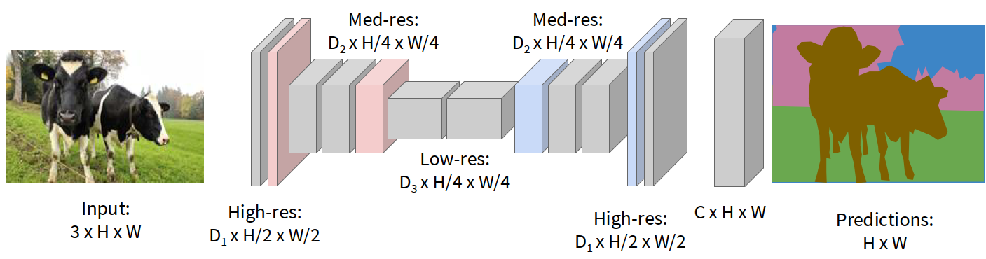
Downsampling and upsampling

A practical FCN-style segmentation network does:

downsample the image several times
process lower-resolution feature maps
upsample features back to full resolution
predict a per-pixel class map

Downsampling can be done by:

pooling
strided convolution

Upsampling can be done by:

nearest-neighbor / unpooling
max unpooling
transposed convolution

In-network upsampling

1. Unpooling / nearest neighbor

Simplest way:

copy each low-resolution value into a larger region
no learned parameters

For example, a $2 \times 2$ input can be expanded into a $4 \times 4$ output by replication.

2. Bed of nails

Another simple option:

place original values at sparse locations
fill the rest with zeros

This is also not learnable.

3. Max unpooling

If downsampling was done by max pooling:

remember the positions of maxima in the pooling layer
when upsampling, place values back only at those recorded positions

This partially restores spatial structure.

4. Transposed convolution

A learnable upsampling method is transposed convolution.

The understanding of transposed convolution:

ordinary strided convolution can be seen as learnable downsampling
transposed convolution reverses this idea and becomes learnable upsampling
each input value places a weighted copy of the filter into the output
overlapping contributions are summed together

So transposed convolution is not simply “inverse convolution” in the strict algebraic sense. It is better understood as a learned operator that increases spatial resolution.

U-Net

A very important segmentation architecture is U-Net.

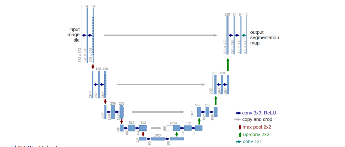
understanding of U-Net:

the left side is the downsampling / encoder path
the right side is the upsampling / decoder path
skip connections copy high-resolution features from encoder to decoder
decoder combines coarse semantic information with fine spatial information

Why skip connections help:

encoder deeper layers have strong semantics but poor spatial detail
early layers have fine local structure
concatenating encoder features into decoder helps recover sharp boundaries

Summary of semantic segmentation

Semantic segmentation:

predicts one category for each pixel
does not separate different instances of the same class
focuses on semantic labels, not object identity

Example:

two cows in one image may both simply be labeled as cow
the output does not need to distinguish cow A from cow B

Object Detection

Single-object detection

If there is only one object, the problem is relatively simple.

We can predict:

class scores for the object category
bounding box coordinates $(x, y, w, h)$

This is basically:

classification + localization

Loss design:

softmax loss for the class label
regression loss (such as L2 / smooth L1) for box coordinates
combine them into a multitask loss

So object detection naturally involves multiple objectives at the same time.

For multiple objects, the output size is not fixed:

different images have different numbers of objects
each object has its own class and bounding box

So a naive fixed-size output layer becomes awkward.

Sliding window over crops:

take many crops / windows from the image
run a CNN on each crop
classify it as object / background

Problem:

need to evaluate huge numbers of windows
must search over locations, scales, and aspect ratios
computationally very expensive

region proposals:

candidate image regions likely to contain objects
then only run the detector on these candidate regions

This was the key idea behind the R-CNN family.

R-CNN

Pipeline of R-CNN:

generate ~2000 region proposals by selective search or another proposal method
warp each proposed region to a fixed size
run each region independently through a ConvNet
classify each region
regress bounding-box corrections

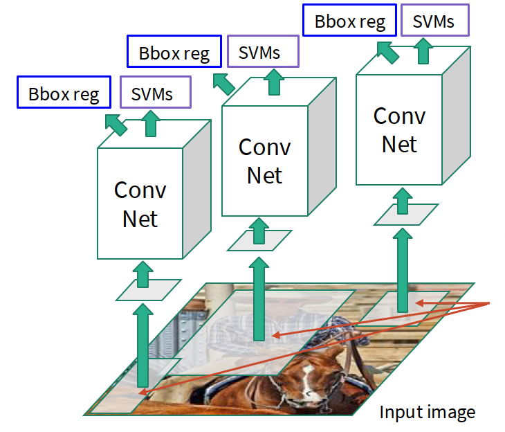
The understanding of R-CNN:

good idea: convert detection into classification on candidate regions
bad part: thousands of proposals mean thousands of CNN forward passes

Main problem:

very slow
huge repeated computation

Fast R-CNN

Fast R-CNN improves this by sharing convolution.

Basic idea:

run the whole image once through the backbone CNN
get feature maps for the image
project each RoI onto the feature map
crop and resize region features
classify each region and regress box offsets This is much better because:
heavy convolution is shared across all regions
only the later region-specific head is run per proposal

RoI Pool and RoI Align

In Fast R-CNN, we need a way to convert variable-size regions on the feature map into fixed-size features.

RoI Pool

RoI Pool does:

project proposal onto the feature map
snap region boundaries to grid cells
divide region into small subregions
max-pool inside each subregion

This gives fixed-size region features.

But there is a problem:

snapping to grid introduces misalignment
small localization errors matter, especially for masks

RoI Align

RoI Align fixes this by:

not snapping to grid
sampling regularly using bilinear interpolation
preserving more accurate spatial alignment

Region Proposal Network (RPN)

Instead of hand-designed proposal algorithms, we can let the CNN predict proposals itself.

A Region Proposal Network does:

place anchor boxes at each feature-map location
predict whether each anchor contains an object
regress box offsets for positive anchors
rank proposals by objectness score
keep top proposals

In practice:

use multiple anchors of different scales / aspect ratios
output objectness + box transform for each anchor

This makes proposal generation part of the network itself.

Faster R-CNN

The understanding of Faster R-CNN:

first stage: propose candidate boxes
second stage: classify proposals and refine boxes
this is why Faster R-CNN is called a two-stage detector

Typical losses:

RPN object / background loss
RPN box regression loss
final classification loss
final box regression loss

Single-stage detectors: YOLO / SSD / RetinaNet

Another direction is to skip the second stage and predict detections directly.

High-level idea: divide the image into a grid, and directly predict boxes + confidence + class scores.

Within each grid cell:

predict whether there is an object
regress bounding boxes
predict class probabilities

Advantages:

very fast
one forward pass
suitable for real-time applications

Tradeoff:

often less accurate than strong two-stage detectors
especially for small / crowded objects in older versions

DETR

A more modern idea is to use Transformers directly for object detection.

DETR:

outputs a set of predicted boxes directly
does not use anchors
does not use box proposal stages in the old style
matches predictions to ground truth with bipartite matching
trains box coordinates end-to-end

The understanding of DETR:

object detection becomes a set prediction problem
Transformer decoder queries correspond to possible objects
each query tries to explain one object or “no object”

This is conceptually elegant because it removes many hand-designed detection components.

Detection tradeoffs

In object detection, there are many design choices:

backbone architecture
image size
proposal mechanism
two-stage or single-stage
anchor design
speed vs accuracy balance

A broad empirical takeaway:

Faster R-CNN: slower but usually more accurate
SSD / YOLO: faster but historically a bit less accurate
bigger / deeper backbones often improve performance

Instance Segmentation

Instance segmentation combines:

object detection
per-instance mask prediction

So unlike semantic segmentation:

we do not only label pixels
we also separate different instances of the same class

Example:

two dogs should become two different masks, not one shared “dog” region

Mask R-CNN

Mask R-CNN extends Faster R-CNN by adding a mask head.

Pipeline:

backbone CNN + RPN generate proposals
RoI Align extracts fixed-size aligned region features
one branch predicts class scores
one branch predicts box coordinates
one small mask network predicts a binary mask for each class

Typical output of mask head:

per-RoI mask such as $28 \times 28$
one mask per class
during inference, keep the mask corresponding to the predicted class

The understanding of Mask R-CNN:

Faster R-CNN already tells us where the object is
mask head tells us which pixels inside the box belong to the object
RoI Align is crucial because masks are sensitive to pixel-level alignment

Visualization and Understanding

Besides building models, we also want to understand:

what the model learns
which features it uses
which image regions matter for a prediction

For the first convolution layer, filters can be directly visualized because:

they usually have 3 input channels (RGB)
the filter itself can be displayed as a small image

Typical result:

edge detectors
color blobs
oriented patterns
simple texture filters

The understanding of first-layer filters:

early CNN layers learn low-level visual primitives
these are similar across many architectures
later layers become more abstract and are harder to visualize directly

Saliency maps

A saliency map asks:

Which pixels matter most for a particular class score?

Method:

do a forward pass and compute the class score $S_c$
compute gradient of the class score with respect to input pixels
take absolute value and often max over RGB channels

Mathematically: $$ M = \max_{ch} \left| \frac{\partial S_c}{\partial I} \right| $$

where $I$ is the input image.

The understanding of saliency maps:

if a pixel has large gradient magnitude, changing that pixel changes the class score a lot
therefore that pixel is important for the prediction

CAM (Class Activation Mapping)

CAM gives a class-specific heatmap from convolutional features.

Setup:

suppose the last convolution feature map is $f \in \mathbb{R}^{H \times W \times K}$
global average pooling gives pooled features $F \in \mathbb{R}^{K}$
final linear classifier has weights $w \in \mathbb{R}^{K \times C}$

Then $$ F_k = \frac{1}{HW} \sum_{h,w} f_{h,w,k} $$

and class score $$ S_c = \sum_k w_{k,c} F_k $$

Substituting gives $$ S_c = \frac{1}{HW} \sum_{h,w} \sum_k w_{k,c} f_{h,w,k} $$

So define the class activation map $$ M^c_{h,w} = \sum_k w_{k,c} f_{h,w,k} $$

This heatmap tells us which spatial locations support class $c$.

Limitation of CAM:

only works naturally for the last convolution layer in a specific architecture form
requires global average pooling + linear classifier structure

Grad-CAM

Grad-CAM generalizes CAM to arbitrary layers.

Steps:

choose any layer with activations $A \in \mathbb{R}^{H \times W \times K}$
compute gradient of class score with respect to activations $$ \frac{\partial S_c}{\partial A} $$
global-average-pool these gradients over spatial dimensions to get channel weights $$ \alpha_k = \frac{1}{HW} \sum_{h,w} \frac{\partial S_c}{\partial A_{h,w,k}} $$
combine activations using these weights $$ M^c_{h,w} = \operatorname{ReLU}\left(\sum_k \alpha_k A_{h,w,k}\right) $$

The understanding of Grad-CAM:

gradients tell us which channels matter for the chosen class
activations tell us where those channels are active
combine them to get a class-specific localization heatmap

Guided backprop

Another interpretation method is guided backprop.

Basic idea:

pick a specific intermediate neuron / channel
compute gradient of that neuron with respect to image pixels
when backpropagating through ReLU, keep only positive gradients

This tends to produce sharper-looking visualizations than plain backprop.

Visualizing ViT features

For ViTs, interpretability often comes more naturally from attention:

attention maps show which patches look at which other patches
patch tokens preserve sequence structure
we can visualize how different heads attend over the image

This is one reason transformer-style models are often easier to inspect in terms of token interaction.

Glossary

semantic segmentation n. 语义分割
instance segmentation n. 实例分割
object detection n. 目标检测
localization n. 定位
bounding box n. 边界框
multitask loss n. 多任务损失
region proposal n. 区域候选 / 候选框
RoI (Region of Interest) n. 感兴趣区域
objectness n. 含有目标的概率
anchor box n. 锚框
transposed convolution 转置卷积 / 反卷积
unpooling 反池化 / 上采样
skip connection n. 跳跃连接
saliency map n. 显著图
class activation map (CAM) n. 类激活图
Grad-CAM n. 基于梯度的类激活图
guided backprop n. 引导反向传播