From Seq2Seq RNN to Attention
For sequence-to-sequence tasks like machine translation, we may want to input one sequence and output another sequence.
- Input: English sentence
- Output: Italian / French sentence
- The lengths of input and output sequences may be different.
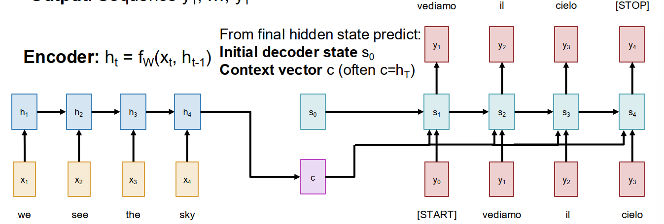
A classic solution before Transformers was Encoder - Decoder RNN.
- The encoder RNN reads the input sequence and updates hidden states
- The decoder RNN generates output tokens one by one
- We often use the final hidden state of encoder as a context vector $c$
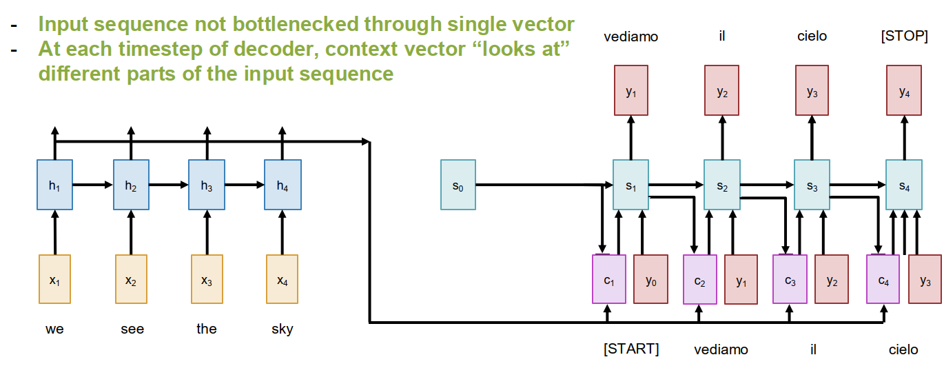
The bottleneck problem
The basic Seq2Seq RNN summarizes the whole input sequence into one fixed-size context vector $c$.
- This may work for short sequences.
- But for very long sequences, it is difficult to compress everything into one vector.
- Therefore, the information of the input sequence is bottlenecked by $c$.
High-level idea: Instead of forcing the whole input into one vector, let the decoder look back at the whole input sequence at each step.
Attention in Seq2Seq
For each decoder timestep $t$, we compare the previous decoder hidden state $s_{t-1}$ with every encoder hidden state $h_i$.
Step 1: alignment scores: We compute scalar alignment scores $$ e_{t,i} = f_{att}(s_{t-1}, h_i) $$ where $f_{att}$ can be a learnable function such as a linear layer.
Step 2: attention weights: apply softmax to get attention weights $$ a_{t,i} = \operatorname{softmax}(e_{t,i}) $$ with properties:
- $0 < a_{t,i} < 1$
- $\sum_i a_{t,i} = 1$
Step 3: context vector
We compute the context vector as a weighted sum of encoder hidden states $$ c_t = \sum_i a_{t,i} h_i $$
Step 4: decode with context
The decoder now uses the current context vector $$ s_t = g_U(y_{t-1}, s_{t-1}, c_t) $$
The understanding of attention:
- for each output timestep, the decoder can attend to the relevant parts of the input sequence.
- different output tokens may attend to different input positions.
- the whole mechanism is differentiable, so we can backprop through everything.
- no explicit supervision on alignment is needed.
Visualizing attention
Attention weights are interpretable.
- If the attention map is close to diagonal, the input and output words roughly correspond in order.
- Non-diagonal structure may indicate word reordering.
- Therefore, attention also gives us some understanding of what the model is using.
Attention Layer
The attention mechanism inside Seq2Seq RNN can be abstracted into a more general operator.
Single query version
Inputs:
- Query vector: $q \in \mathbb R^{D_Q}$
- Data vectors: $X \in \mathbb R^{N_X \times D_X}$
Computation:
- Similarities: $$ e_i = f_{att}(q, X_i) $$
- Attention weights: $$ a = \operatorname{softmax}(e) $$
- Output vector: $$ y = \sum_i a_i X_i $$
So the attention layer takes a query and summarizes a set of data vectors into one output vector.
Scaled Dot-Product Attention
A simple choice for similarity is dot product. $$ e_i = q \cdot X_i $$
In practice, we usually use scaled dot-product: $$ e_i = \frac{q \cdot X_i}{\sqrt{D}} $$
Why scale?
- When the dimension is large, dot products can become very large.
- Then softmax may saturate.
- Saturated softmax leads to very small gradients.
- So dividing by $\sqrt{D}$ helps stabilize training.
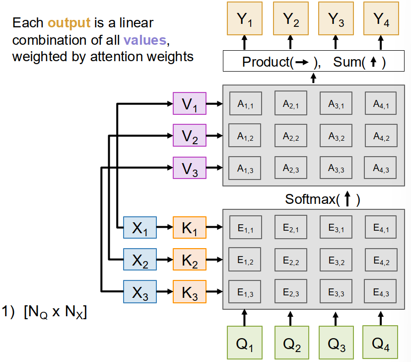
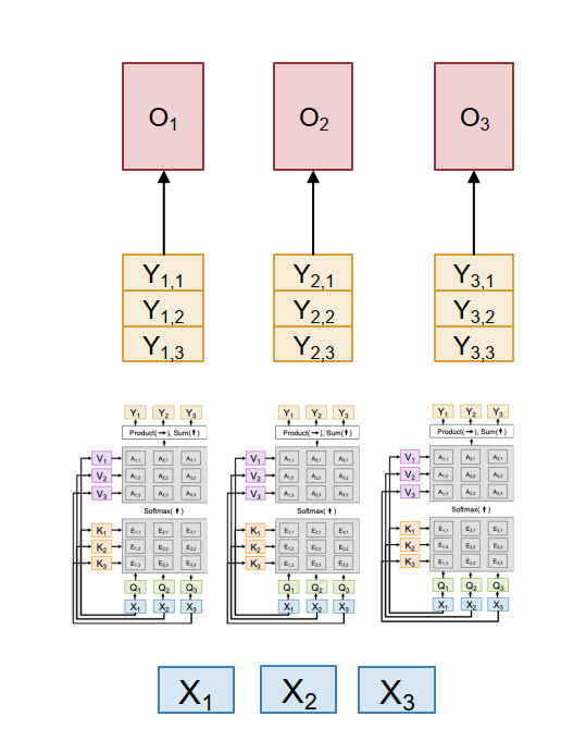
Multiple Queries, Keys and Values
We can generalize attention to multiple queries.
Let
- $Q \in \mathbb R^{N_Q \times D_Q}$ be the query matrix
- $X \in \mathbb R^{N_X \times D_X}$ be the data matrix
Then attention can be written as $$ E = \frac{QX^T}{\sqrt{D_Q}}, \qquad A = \operatorname{softmax}(E), \qquad Y = AX $$
But usually we further separate the role of data vectors into keys and values.
Keys and values
We learn two projections $$ K = XW_K, \qquad V = XW_V $$ where
- $K$ is used for similarity matching with queries
- $V$ is used for constructing outputs
So the final attention formula becomes $$ E = \frac{QK^T}{\sqrt{D_Q}}, \qquad A = \operatorname{softmax}(E), \qquad Y = AV $$
The understanding of keys and values:
- keys decide where to attend
- values decide what information to retrieve
Cross-Attention and Self-Attention
Cross-Attention
In cross-attention:
- queries come from one source
- keys and values come from another source
So each query produces an output by mixing information from another set of vectors.
This is natural in encoder-decoder setting.
- decoder states provide queries
- encoder states provide keys and values
Self-Attention
In self-attention, all queries, keys, and values are computed from the same input vectors $X$.
We learn three projections: $$ Q = XW_Q, \qquad K = XW_K, \qquad V = XW_V $$
Then compute $$ E = \frac{QK^T}{\sqrt{D_Q}}, \qquad A = \operatorname{softmax}(E), \qquad Y = AV $$
This means:
- each input vector produces one query, one key, and one value.
- each output vector is a weighted sum of all value vectors.
- therefore, each input can interact with all other inputs.
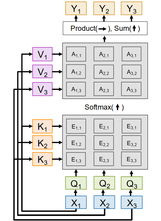
In practice, $Q,K,V$ are often computed in one fused matrix multiplication: $$ [Q\ K\ V] = X[W_Q\ W_K\ W_V] $$
Permutation Equivariance and Positional Encoding
A pure self-attention layer is permutation equivariant.
- If we permute the inputs, then queries, keys, values, similarities, attention weights, and outputs are also permuted in the same way.
- So self-attention itself does not know the order of a sequence.
- In that sense, self-attention works on a set of vectors.
Formally, $$ F(\sigma(X)) = \sigma(F(X)) $$
The problem
For language or time series, order matters.
The solution: positional encoding
We add positional encoding to each input vector.
- It is a vector that depends on the position index.
- After adding it, the model can distinguish different positions.
Masked Self-Attention
Sometimes we do not want an input to look at all other positions.
For autoregressive language modeling, a token should not look ahead to future tokens.
- token 1 can only see token 1
- token 2 can only see tokens 1, 2
- token 3 can only see tokens 1, 2, 3
So we use masking:
- overwrite forbidden similarity entries with $-\infty$
- after softmax, those positions get attention weight $0$
This produces causal / masked self-attention.
Multiheaded Self-Attention
Instead of using one self-attention layer, we often run several self-attention layers in parallel. These are called heads.
If there are $H$ heads:
- each head has its own $W_Q, W_K, W_V$
- each head computes its own attention output
- then we concatenate all head outputs and apply an output projection
If the model dimension is $D$, the head dimension is often $$ D_H = D / H $$ so that input and output dimensions stay the same.
Why multihead?
- different heads may focus on different relations
- some heads may learn local interactions
- some heads may learn long-range interactions
- it increases model capacity without changing the high-level structure
Self-Attention as Four Matrix Multiplies
Multiheaded self-attention can be viewed as four matrix multiplications.
- QKV projection $$ [N \times D][D \times 3HD_H] \Rightarrow [N \times 3HD_H] $$
- QK similarity $$ [H \times N \times D_H][H \times D_H \times N] \Rightarrow [H \times N \times N] $$
- V-weighting $$ [H \times N \times N][H \times N \times D_H] \Rightarrow [H \times N \times D_H] $$
- Output projection $$ [N \times HD_H][HD_H \times D] \Rightarrow [N \times D] $$
So although attention looks conceptually rich, most of the computation is still large matrix multiplication.
Complexity of Self-Attention
The main problem of self-attention is the $N \times N$ attention matrix.
Compute complexity
The compute of self-attention grows as $$ O(N^2) $$ with sequence length $N$.
Memory complexity
The memory also grows as $$ O(N^2) $$ if we explicitly store the whole attention matrix.
This becomes expensive for very long sequences.
Flash Attention
Flash Attention avoids storing the full attention matrix explicitly.
- It computes the softmax-weighted value aggregation in a fused way.
- Therefore, memory can be reduced to approximately $O(N)$.
- This makes much larger sequence length possible in practice.
Three Ways of Processing Sequences
Recurrent Neural Network
- works on 1D ordered sequences
- theoretically good at long sequences: $O(N)$ compute and memory
- but not parallelizable because hidden states must be computed sequentially
Convolution
- works on $N$-dimensional grids
- outputs can be computed in parallel
- but long-range interaction is hard because receptive field grows slowly
Self-Attention
- works on sets of vectors
- each output depends directly on all inputs
- highly parallelizable
- but expensive because of quadratic complexity
Transformer Block
The Transformer uses self-attention as its core primitive.
A standard transformer block contains:
- Multiheaded self-attention
- Residual connection
- Layer normalization
- MLP / FFN on each vector independently
- Another residual connection
- Another layer normalization
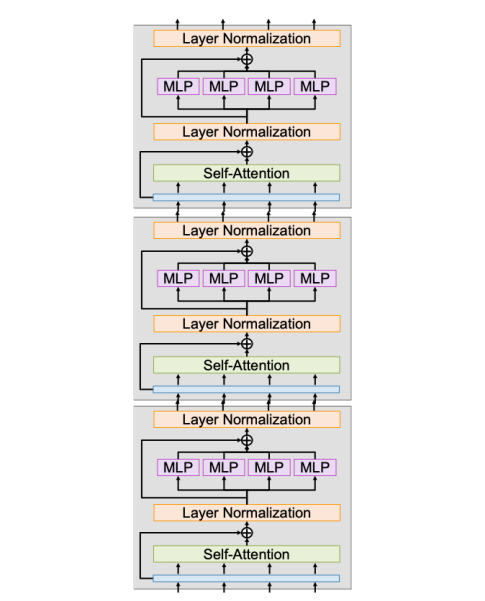
Important understanding
- Self-Attention is the only part where different vectors directly interact.
- LayerNorm and MLP operate on each vector independently.
- Most computation is just matrix multiplications:
- 4 from self-attention
- 2 from the MLP
MLP / FFN
The MLP is usually a two-layer feed-forward network applied independently to each vector: $$ D \Rightarrow 4D \Rightarrow D $$
This means:
- self-attention mixes information across tokens
- MLP increases nonlinear processing capacity for each token
A full Transformer is just a stack of many identical transformer blocks.
Transformers for Language Modeling
For language modeling:
- Learn an embedding matrix of shape $[V \times D]$ to map tokens to vectors.
- Add positional encoding.
- Pass the sequence through many transformer blocks.
- Use masked attention so each token only sees previous tokens.
- At the end, project from $D$ to vocabulary size $V$.
- Apply softmax and cross-entropy loss to predict the next token.
The understanding of LLMs from this lecture:
- an LLM is essentially a masked transformer for next-token prediction.
- the embedding matrix converts tokens into vectors.
- the output projection converts vectors back to vocabulary scores.
Vision Transformers (ViT)
Transformers can also process images.
Main idea: Instead of treating the image as a grid for CNN filters, we split the image into patches and treat each patch like a token.
For example, for a $224 \times 224 \times 3$ image:
- break it into $16 \times 16 \times 3$ patches
- flatten each patch into a vector of length $768$
- apply a linear transform $768 \Rightarrow D$
- use the resulting $D$-dimensional patch vectors as transformer inputs
Additional details:
- Use positional encoding to tell the model the 2D location of each patch.
- Do not use causal masking, because every patch can attend to every other patch.
- The transformer outputs one vector per patch.
- Then we can average pool the patch outputs and use a linear layer for classification.
Common Tweaks of Transformers
Although the transformer architecture has not changed too much, some modifications have become common.
Pre-Norm
Move normalization before self-attention and MLP, inside the residual branches.
- training is more stable
- optimization is usually easier
RMSNorm
Replace LayerNorm with RMSNorm.
Given input $x \in \mathbb R^D$, RMSNorm computes $$ y_i = \frac{x_i}{\operatorname{RMS}(x)} \gamma_i $$ where $$ \operatorname{RMS}(x) = \sqrt{\epsilon + \frac{1}{N} \sum_{i=1}^{N} x_i^2} $$
Compared with LayerNorm:
- it does not subtract mean
- it is a bit simpler
- it is often more stable in practice
SwiGLU MLP
Instead of the classic MLP $$ Y = \sigma(XW_1)W_2 $$ we can use SwiGLU: $$ Y = \sigma(XW_1) \odot XW_2 ; W_3 $$
This adds a gating effect and often improves performance.
Mixture of Experts (MoE)
Instead of one MLP, learn $E$ different experts.
- each token is routed only to $A < E$ active experts
- parameters increase a lot
- compute increases much less
So MoE can greatly expand model size without increasing computation proportionally.
Glossary
- primitive n. 基本操作;底层构件
- permutation equivariant 置换等变的
- positional encoding n. 位置编码
- masked attention n. 掩码注意力
- causal adj. 因果的
- head dim 注意力头维度
- receptive field 感受野
- routing n. 路由;分配
- expert n. 专家模块