Sequence Modeling

So far, vanilla neural networks usually assume fixed-size input and fixed-size output.

But many real tasks are naturally in the form of sequence:

• image $\to$ sequence of words
• sequence of video frames $\to$ one action class
• sequence of video frames $\to$ sequence of words
• sequence $\to$ sequence with the same length

Common sequence modeling forms:

• one to many: image captioning
• many to one: action classification from video
• many to many: video captioning / frame-level classification

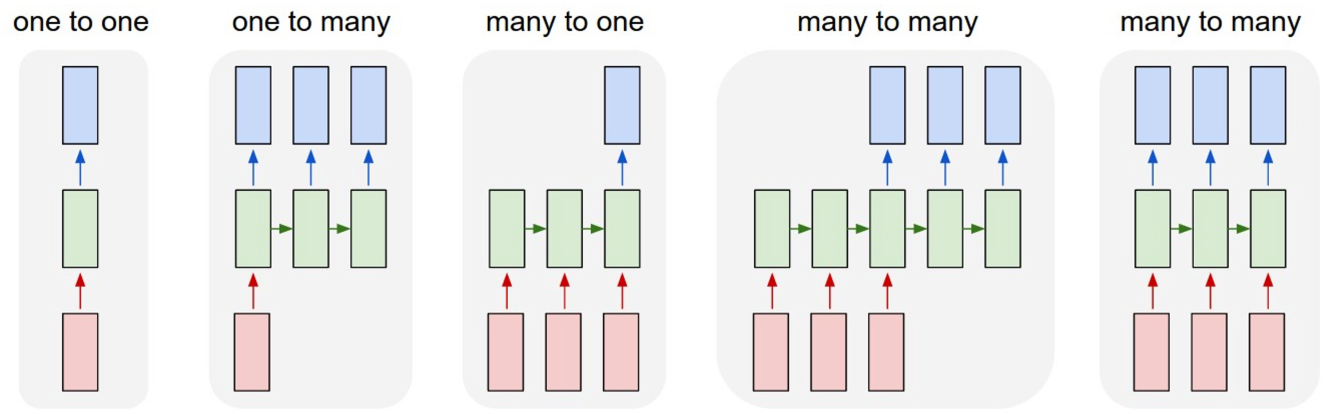
The key difference is that the sequence length can be variable.

Recurrent Neural Networks

High-level idea: RNN has an internal state / hidden state that is updated when the sequence is processed.

So at time step $t$, the new hidden state depends on:

• previous hidden state $h_{t-1}$
• current input $x_t$

A general formulation is: $$ h_t = f_h(W_{hh} h_{t-1} + W_{xh} x_t) $$ $$ y_t = f_y(W_{hy} h_t) $$

where:

• $h_t$ is the hidden state at time step $t$
• $x_t$ is the input at time step $t$
• $y_t$ is the output at time step $t$
• $W_{hh}$ transforms previous hidden state to current hidden state
• $W_{xh}$ transforms current input to hidden state space
• $W_{hy}$ transforms hidden state to output space

Important property:

• the same function is used at every time step
• the same weights are reused at every time step

This is why RNN can process variable-length input without increasing model size.

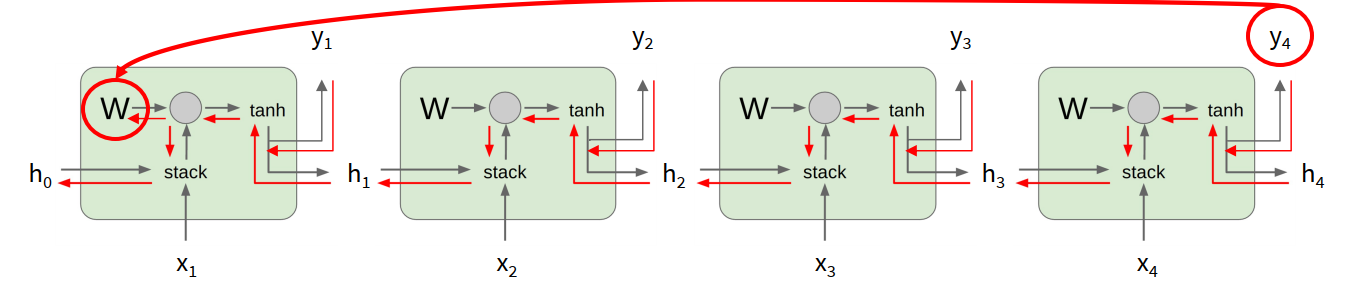
Unrolled RNN

The compact recurrent diagram is sometimes not easy to reason about. So we often unroll the RNN across time.

Then the dependency becomes explicit:

• $h_1$ depends on $h_0$ and $x_1$
• $h_2$ depends on $h_1$ and $x_2$
• $h_3$ depends on $h_2$ and $x_3$
• …

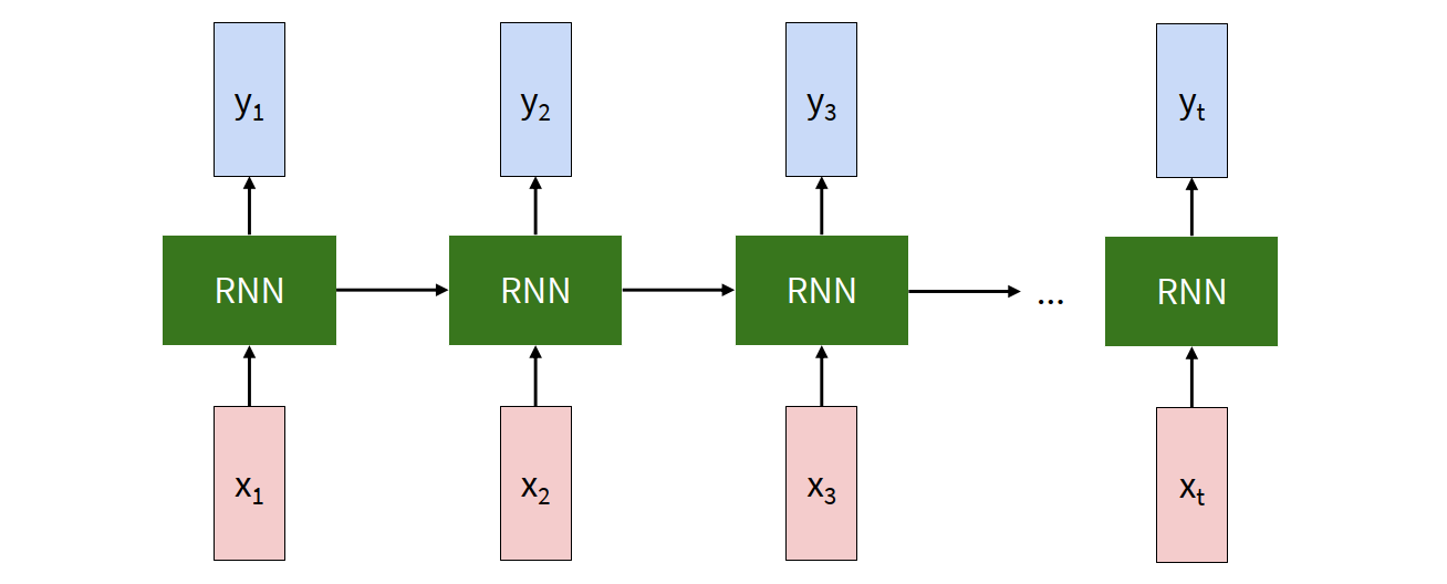
This view is especially useful for understanding forward pass and backpropagation through time.

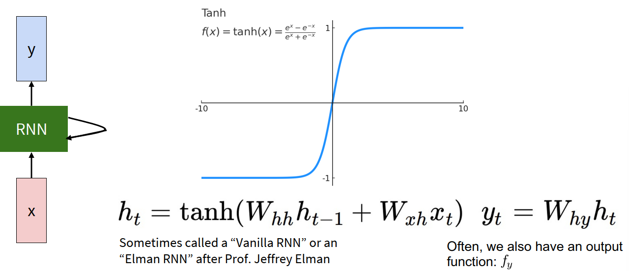
Vanilla RNN

A standard vanilla RNN often uses tanh: $$ h_t = \tanh(W_{hh} h_{t-1} + W_{xh} x_t) $$ $$ y_t = W_{hy} h_t $$

Why tanh is commonly used:

• it is zero-centered
• it can represent both positive and negative values
• it is bounded in $[-1, 1]$

But this bounded nonlinearity also contributes to vanishing gradients later.

toy example: manually build an RNN to detect repeated 1s in a binary sequence.

Example task:

• input: $0,1,0,1,1,1,0,1,1,\dots$
• output: give $1$ when there are two consecutive 1s, otherwise output $0$

This is a many to many problem.

What should the hidden state remember?

To decide whether the current output should be 1, the model mainly needs:

• the current input
• the previous input

So the hidden state can store: $$ h_t = (\text{Current}, \text{Previous}, 1) $$

The constant 1 is added to make output computation easier.

We initialize: $h_0 = (0,0,1)$ For simplicity, the lecture uses ReLU instead of tanh in this toy construction.

Hand-crafted weights

The hidden state update is: $$ h_t = \operatorname{ReLU}(W_{hh} h_{t-1} + W_{xh} x_t) $$ $$ y_t = \operatorname{ReLU}(W_{hy} h_t) $$

A valid construction is: $$ W_{xh} = \begin{bmatrix}1\0\0\end{bmatrix}, \qquad W_{hh} = \begin{bmatrix} 0 & 0 & 0 \ 1 & 0 & 0 \ 0 & 0 & 1 \end{bmatrix}, \qquad W_{hy} = \begin{bmatrix}1 & 1 & -1\end{bmatrix} $$

The intuition:

• $W_{xh}$ writes the current input into the first entry of the hidden state
• the second row of $W_{hh}$ copies the previous “current” value into the new “previous” slot
• the third row of $W_{hh}$ keeps the constant 1

Therefore the output becomes: $$ y_t = \max(\text{Current} + \text{Previous} - 1, 0) $$

So only when both current and previous are 1, the output becomes 1.

This example is useful because it shows:

• what the hidden state is storing
• what each weight matrix is doing
• how the output is produced from the hidden state

Computational Graph and Shared Weights

When an RNN is unrolled in time, it looks like a deep computational graph.

But unlike an ordinary deep network, the weight matrix $W$ is shared across all time steps.

That means:

• conceptually, each step contributes a gradient to the same parameter
• practically, the total gradient for that parameter is the sum over time steps

Different task forms:

• many to many: one output for each input, maybe one loss for each time step
• many to one: only use final state or pooled states for one final output
• one to many: start from one input, then generate a sequence

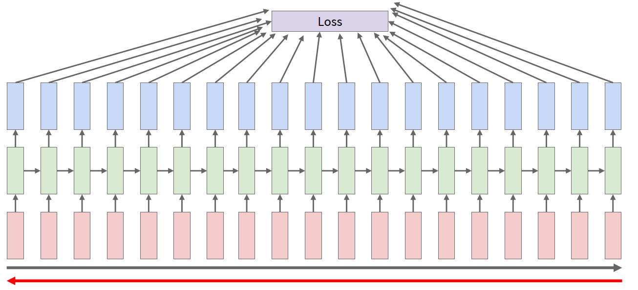
Backpropagation Through Time

Backpropagation Through Time (BPTT): forward through the whole sequence to compute the loss, then backward through the whole sequence to compute the gradient.

In many-to-many tasks, the total loss can be written as: $$ L = \sum_t L_t $$

Because the same weights are reused at every time step, gradients from different time steps are accumulated onto the same parameter.

Truncated BPTT

In practice, sequences may be too long.

If we backprop through the whole sequence:

• memory cost becomes very high
• computation becomes very slow

So a common trick is truncated BPTT.

High-level idea:

• carry the hidden states forward for the full sequence
• but only backpropagate through a smaller time window

This is essentially chunking the sequence into manageable pieces.

Benefits:

• lower memory cost
• more practical training on long sequences

Cost:

• gradient is only approximate compared with full BPTT
• long-range dependency across chunks is weakened

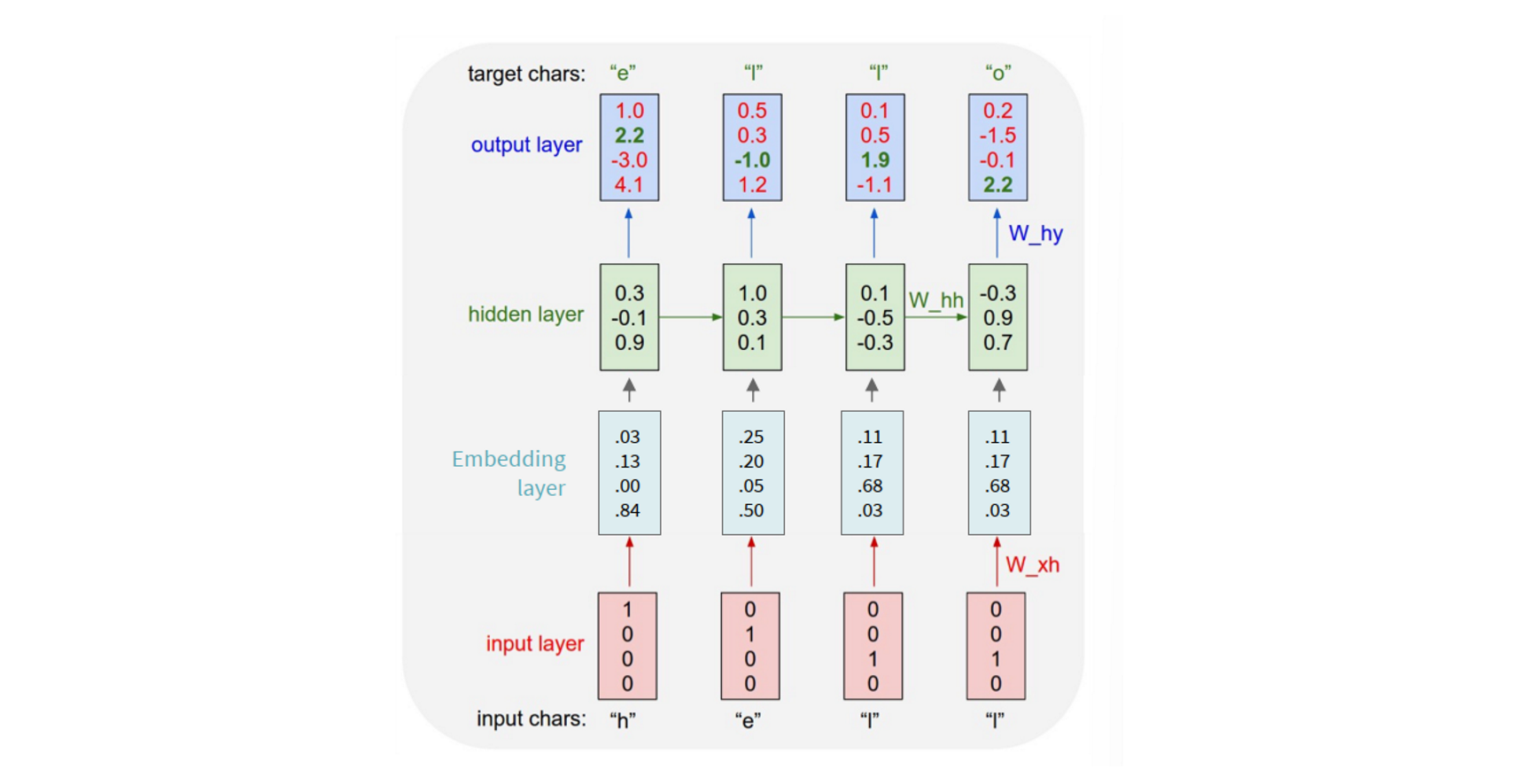
Character-level Language Model

A practical use of RNN is language modeling.

Example vocabulary: $[h, e, l, o]$

Example sequence: $\text{“hello”}$

At each time step:

• input the current character
• predict the next character

So this is essentially a time-step-wise classification problem.

One-hot input and softmax output

Each character can be represented as a one-hot vector.

Example:

• $h \to [1,0,0,0]$
• $e \to [0,1,0,0]$
• $l \to [0,0,1,0]$
• $o \to [0,0,0,1]$

The output logits are passed through softmax to produce a probability distribution over the vocabulary.

At training time, we compare the predicted distribution with the ground-truth next character.

Sampling at test time

At test time:

• sample one character from the output distribution
• feed it back as the next input
• repeat until the sequence is finished

So generation is autoregressive.

If we always choose the maximum probability, that is greedy decoding. In practice, sampling is often better because it gives more diverse outputs.

Embedding layer

Using one-hot vectors directly is usually not the best formulation.

A common trick is to insert an embedding layer before the RNN.

Key idea:

• multiplying an embedding matrix by a one-hot vector is equivalent to selecting one row / column from the matrix
• therefore each token gets mapped to a learnable dense vector

Why embeddings are useful:

• dense vector input works better than raw discrete index / one-hot representation
• embeddings are learnable
• the model can place similar tokens in nearby vector space

A tiny char-RNN can already generate text that gradually becomes more coherent during training. This is historically important because it already showed the basic recipe of modern language modeling:

• predict next item in a sequence
• feed generated item back into the model
• train on huge corpora without manual labeling

Interpretable Hidden Cells

One very interesting thing in RNNs is that some hidden units can become somewhat interpretable.

Examples shown in lecture:

• quote detector cell: activates inside quotation marks
• line length tracking cell: tracks when a newline may come
• if statement cell: tracks whether we are inside an if block
• quote/comment cell: detects whether we are inside comment / quote structure
• code depth cell: tracks code indentation depth

This suggests that some hidden states are automatically learning useful discrete-like structural signals.

RNN Tradeoffs

Advantages:

• can process inputs of arbitrary length
• model size does not increase with sequence length
• the same weights are reused at each time step
• in theory, information from many steps back can influence the current state
• at inference / recurrence level, compute scales linearly with sequence length

Disadvantages:

• recurrent computation is inherently sequential, so it is slow
• training is hard because later states depend on all previous states
• hidden state has fixed size, so long-range information is hard to preserve in practice
• gradients can vanish or explode over many time steps

Computer Vision Applications of RNNs

Before transformers dominated, RNNs were widely used in vision-language tasks.

Examples:

• image captioning
• visual question answering (VQA)
• visual dialog
• vision-language navigation

Image captioning

A common formulation is:

• use a CNN to encode the image
• use the visual feature as an extra input to the RNN hidden state update
• generate one word/token at a time until an <END> token is sampled

A simple modified hidden state formula is: $$ h_t = \tanh(W_{xh} x_t + W_{hh} h_{t-1} + W_{ih} v) $$

where $v$ is the visual feature from the image encoder.

These systems already worked quite well for simple scenes, but also had obvious failure modes:

• hallucinating objects that are common in a scene
• confusing visually similar contexts
• over-relying on dataset co-occurrence bias

Multilayer RNNs

Just like CNNs or MLPs, RNNs can also be stacked in depth.

High-level idea:

• each layer has its own hidden states across time
• recurrence happens within the same layer over time
• output of a lower layer becomes input to the upper layer

So RNN has two axes: time and depth.

This makes the computation graph much more expensive than a shallow recurrent model.

Gradient Flow in Vanilla RNN

The core training problem of vanilla RNN is gradient flow across many time steps.

Suppose: $$ h_t = \tanh(W_{hh} h_{t-1} + W_{xh} x_t) $$

Then during backpropagation, gradients repeatedly multiply by:

• the derivative of tanh
• the recurrent weight matrix $W_{hh}$

Why gradients vanish

The derivative of tanh is at most 1, and usually less than 1.

So across many time steps, repeated multiplication tends to shrink gradients.

This leads to vanishing gradients.

Why gradients explode

Even if we ignore the nonlinearity, repeated multiplication by $W_{hh}$ can still be problematic.

The key is the largest singular value of the matrix:

• if largest singular value $> 1$, gradients may explode
• if largest singular value $< 1$, gradients may vanish

So the recurrent chain is unstable over long time horizons.

Gradient clipping

For exploding gradients, a common trick is gradient clipping.

High-level idea:

• if the gradient norm is too large, rescale it

This helps stabilize training, but it does not solve vanishing gradients.

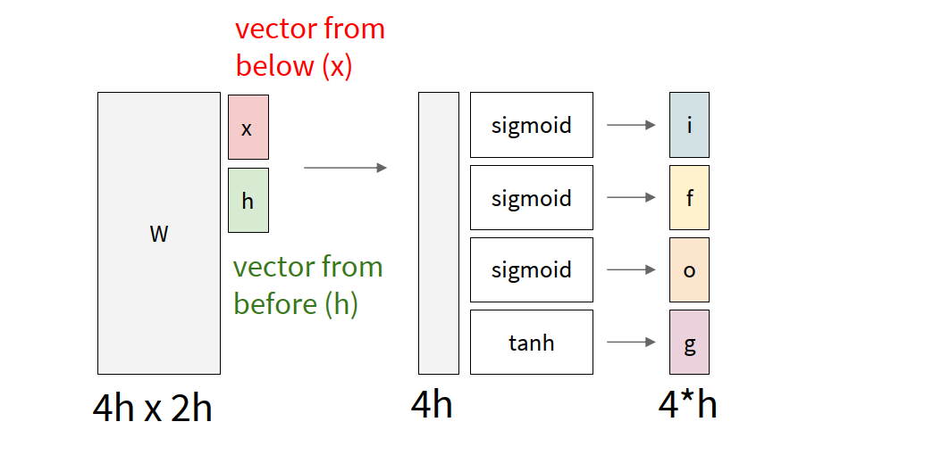
Long Short-Term Memory (LSTM)

LSTM is a more complicated RNN variant designed to make long-term information flow easier.

Instead of only one hidden state, LSTM introduces:

• cell state
• hidden state
• several gates controlling write / forget / reveal behavior

The four common gates are:

• $i$: input gate — whether to write to the cell
• $f$: forget gate — whether to erase old cell information
• $o$: output gate — how much cell information to reveal
• $g$: candidate content to write into the cell

The most important idea is that LSTM creates a more direct pathway for information flow in the cell state.

So from $c_t$ back to $c_{t-1}$, the gradient mainly goes through elementwise multiplication by the forget gate, instead of repeated matrix multiplication plus tanh at every step.

This makes long-range gradient flow much easier.

So compared with vanilla RNN:

• vanilla RNN has to keep information by repeatedly applying the same unstable transformation
• LSTM gives the model a more explicit mechanism to keep / erase / expose information

But LSTM does not completely guarantee no vanishing / exploding gradients. It only makes long-term dependency learning much easier in practice.

important intuition:

• in ResNet, skip connections help information pass across depth
• in LSTM, cell-state pathway helps information pass across time

So both ideas create an easier path for signal propagation.

Modern RNNs

Although vanilla RNNs are old, the hidden-state idea did not disappear.

Modern architectures such as RWKV and Mamba can also be viewed in the broad direction of recurrent / state-space modeling.

Main attractions:

• unlimited context length in principle
• linear scaling with sequence length
• hidden-state style sequential summary of the past

So current research is in some sense trying to get the best of both worlds:

• transformer-level performance
• recurrent/state-space efficiency on long sequences

Glossary

• recurrent adj. 循环的，递归的
• sequence n. 序列
• hidden state n. 隐状态
• unroll v. 展开（计算图）
• recurrence n. 递推，递归关系
• autoregressive adj. 自回归的
• one-hot adj. 独热的
• embedding n. 嵌入向量
• interpretable adj. 可解释的
• singular value n. 奇异值
• clipping n. 裁剪
• gate n. 门控
• captioning n. 图像描述生成
• hallucination n. 幻觉，虚构内容
• state space model n. 状态空间模型