CNN Structure
Components of CNNs:
- Convolution layers
- pooling layers
- fully connected layers
- normalization layers
- dropout
- activation functions
Normalization Layers
High-level idea: Learn parameters that let us scale / shift the input data
LayerNorm: For $N$ samples with $D$ charatersitics $x \in \mathbb R^{N \times D}$
- Calculate mean $\mu$ and standard deviation $\sigma$ $\in \mathbb R^{N\times 1}$ for each sample.
- Learn parameters applies to each sample $\gamma, \beta \in \mathbb R^{1 \times D}$ for each charateristic.
- We first normalize the input data, then scale and shift each sample using learned parameters $y = \gamma (x - \mu) / \sigma + \beta$.
Normalization Method:
- the source of mean $\mu$ and standard deviation $\sigma$ $\in \mathbb R^{N\times 1}$ can be different.
- BatchNorm: calculate for each channel
- LayerNorm: calculate for each sample
- InstanceNorm: calculate for each image
- GroupNorm: calculate for each “grouped channel” in each sample.
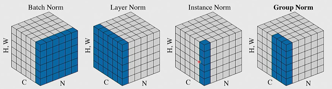
But for scaling and shifting, the parameters are learned. $\gamma$ and $\beta$ usually act on each characteristic or channel (the dimension labeled “C” ).
Dropout
In each forward pass, randomly set some neurons to zero.
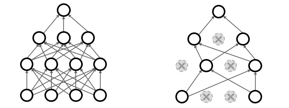
Probability of dropping $p$ is a hyperparameter, usually set as $0.5$ or $0.25$.
The understanding of dropout:
- a method of generalization. The goal is to make it harder for the model to learn the training data so that the generalization ability is better (empirically).
- dropout forces the network to have a redundant representation, so that even when some features are dropped, the model can output the correct label.
- dropout avoid the model to place some of the features heavily.
At backprop:
- For dropped neurons, we don’t need to traverse the path passing them. The gradient is $0$.
At test time:
- we won’t drop any of the neurons.
- we must scale any input of the neurons with $p$ to avoid over-activate the neuron and keep them as expected activated as the training time.
Activation Functions
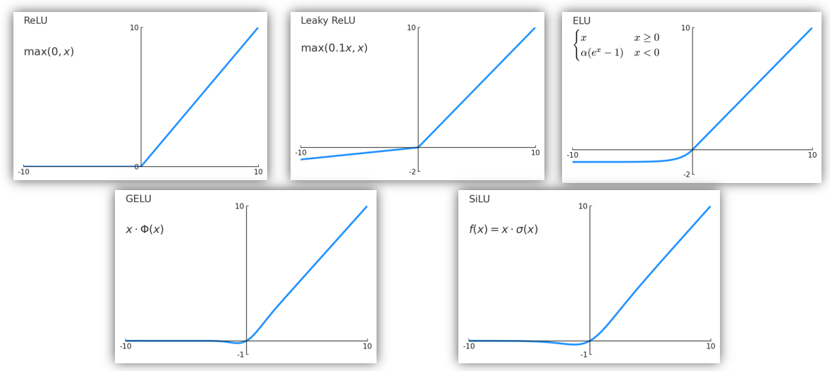
The problem of sigmoid function $\displaystyle \sigma(x) = \frac{1}{1 + e^{-x}}$:
- only saturate in range $(0, 1)$.
- after many layers of sigmoid functions, the gradients become smaller and smaller, especially happening for exceptionally small or large numbers.
The pros and cons of ReLU function $f(x) = \max(0, x)$:
- does not saturate in positive region
- very computationally efficient
- converges much faster than sigmoid in practice.
- is not zero centered output
- will create dead ReLUs when $x < 0$.
- is very popular now in neural networks.
Variations of ReLU:
Activation are generally placed after linear operators (linear layer, conv layer, etc) in CNNs.
CNN Architectures
As the layers of CNN increases, the ability of CNN increases.
- Common Structures: Input - conv - conv - pool - conv - conv - pool - … - Fully Connect - Fully Connect - Softmax - Output
- The deeper models should perform at least well as shallower models.
Small filters are useful: (usually 3 by 3 conv stride 1) can be stacked so that they have the same effective receptive field as larger filters, but fewer parameters need to be trained, and the model is able to more non-linear relationships.
Deeper models are harder to train. It’s not merely overfitting problem but rather optimization problem.
- Cause of the problem: it’s hard for deeper model to learn identity function on single layer and simulate the behavior of shallower models. Deeper models are tend to converge on local minimum.
- Solution: Residual block. We directly take the former computational nodes, skip some layers and link to further nodes. Therefore, the mapping of further nodes can be formalized as $H(x) = f(x) + x$. This make it easier to learn the identity function and simply bypass some of the layers (in that case, weights are all very close to zero).
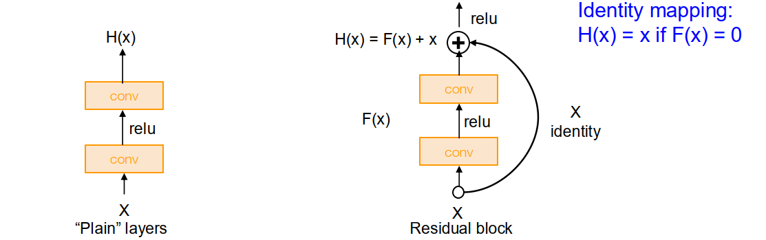
ResNet
Weight Initialization
If the weights are randomly set too large. The activations may explode due to repeating multiplication with no restriction offered by ReLU functions. On the other hand, if the weight are randomly set too small. The activation may become zero quickly.
Kaiming initialization: The weights are randomly set as std = $\sqrt{2/Din}$ with ReLU activation.
CNN Training
Image Preprocessing: normalize each channel. Subtract per-channel mean and divide by per-channel standard deviation.
Randomness:
- During training, we add some kind of randomness $z$. Then actually we are learning the new function $y = f_W (x, z)$.
- During testing, we should calculate the average among all set randomness value. $$y = f(x) = E_z [f(x, z)] = \int_z p(z) f(x, z) \mathrm dz $$
- Example: dropout. During training, we randomly drop activation nodes. While testing, the probability of dropout is $p$, so the activation quantity should multiply by $p$.
Data Augmentation: In this way we get more data and the increase the generalization capability of the model.
- eg. horizontal flips, vertical flip, random crops and scales, color jitter, randomize contrast and brightness, cutout (set random image regions to zero)
Transfer training: If we already have a pre-trained model, we want to train on another new dataset,
- If dataset is small, we can reinitialize weights of the last layer and only train the last layer. The previous layers can already serve as a good feature extractor. We can freeze them from pre-trained model.
- If dataset is large, we should initialized all the layers and fine-tune everything.
| Transfer Training? | Very similar | Vert different |
|---|---|---|
| Small new dataset | Finetune linear classifier on final layer | Try another model or collect more data |
| Large new dataset | Finetune all layers | Finetune all layers or train from scratch |
Choosing Hyperparameters:
- Check initial loss: The initial loss should fall beside the expected value.
- Overfit a small sample: Models should be able to memorize a small sample of training data. Otherwise, there may be some issues in the model.
- Find LR that makes loss go down: The loss is supposed to drop significantly within $\sim 100$ iterations. Good LR to try: $10^{-1}, 10^{-2}, 10^{-3}, 10^{-4}, 10^{-5}$
- Coarse gird of hyperparameters, train for $\sim 1-5$ epochs: So that we quickly sort out obvious bad hyperparams choices.
- Refine grid, train longer.
- Look at loss and accuracy curves (both training and validation)
- If both accuracies goes up with time, we should train longer.
- If train accuracies goes up while val accuracies goes down, that it overfitting. We should increase regularization or get more data.
- If the gap of both accuracies is pretty small. We can train longer and possibly use a bigger model.
- Repeat the process of refining grid, training and optimizing hyperparams.
Random Search: During hyperparam optimization, random search may be more efficient than grid search.
- In random search, we can get more data for every dimensions rather than letting couples of params setting to be almost exactly the same.
- We’ll actually search the hyperparams space more thoroughly whereas rechecking unimportant values for an unimportant hyperparams.
Glossary
- reframe v. 给(图片、照片)换框,重新装裱;再构造;
- saturate v.使湿透,浸透;使充满,使饱和
- albeit conj. 虽然,尽管
- jitter v. 抖动,颤动
- quadrant n. 象限