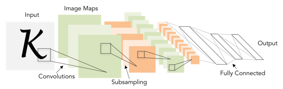
Convolutional Networks
The structure of Convolutional Neural Network:
- Convolution and pooling operators: extract features while respecting 2D image structure.
- Fully-Connected Layers: input the features and output the predict scores.
- all trained with backprop + gradient descent
History:
- First proposed: 1998
- ImageNet
- AlexNet (2012): deep learning developed quickly since then
- in 2012 to 2020: Convnet dominate all vision tasks, including detection, segmentation, image caption (image to text), text-to-image generation,
- Transformers (2017) for language tasks
- Transformers for vision tasks (2021)
Convolution Layer
We maintain the original structure of the image and convolve the filter with the image.
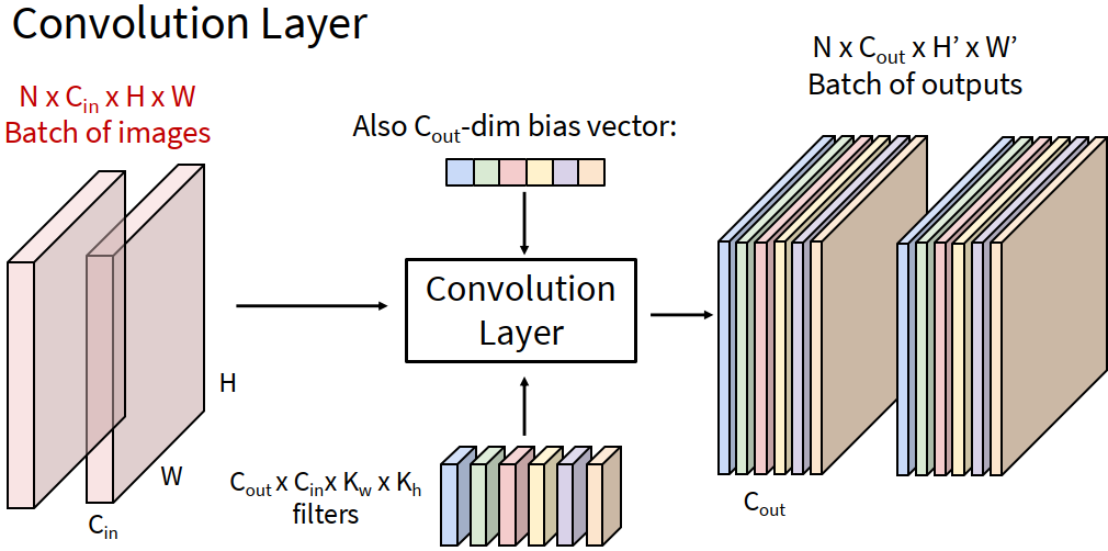
- the bias of the filter are add to the product
- for every filter, we slide everywhere in the image and get the score in the outputs.
- Between the Conv layers, we should add activation functions after Conv function (which is linear).
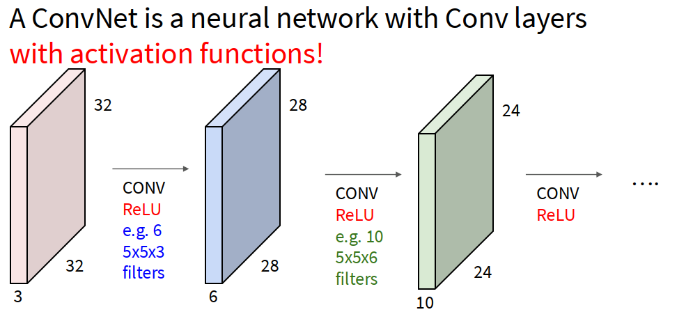
- The random initialization of the filters enable them to recognize different features of the image.
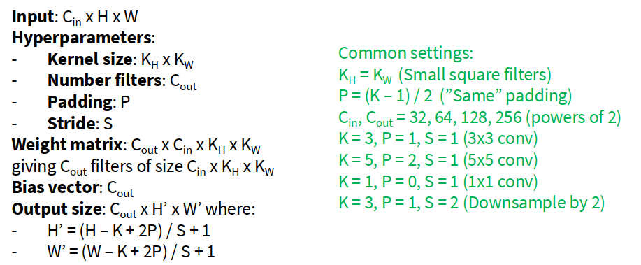
- The feature maps shrink with each layer. We add padding around the input before sliding the filter. To ensure the output have the same size of the input, $\text{padding size} = (\text{filter size} - 1) / 2$.
Receptive Fields:
- Each element in the output depends on a $k \times k$ receptive filed in the input.
- After stacking multiple filters, each successive convolution add $K-1$ to the receptive field size. The size of the $L^{th}$ receptive field size is $1 + L (K - 1)$.
Strided Convolution:
- rather than placing the filter everywhere in the image, we take larger move of the filter when sliding the image. Hence there’s another hyperparameter Stride Length.
- The output size if $(\text{Input size} - \text{Filter Size} + 2 ·\text{Padding}) / \text{Stride} + 1$. It decreases exponentially so there are not too much conv layers.
Other Types of Convolution:
- 1d Convolution
- 3D convolution
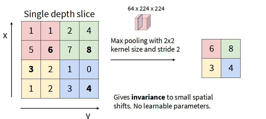
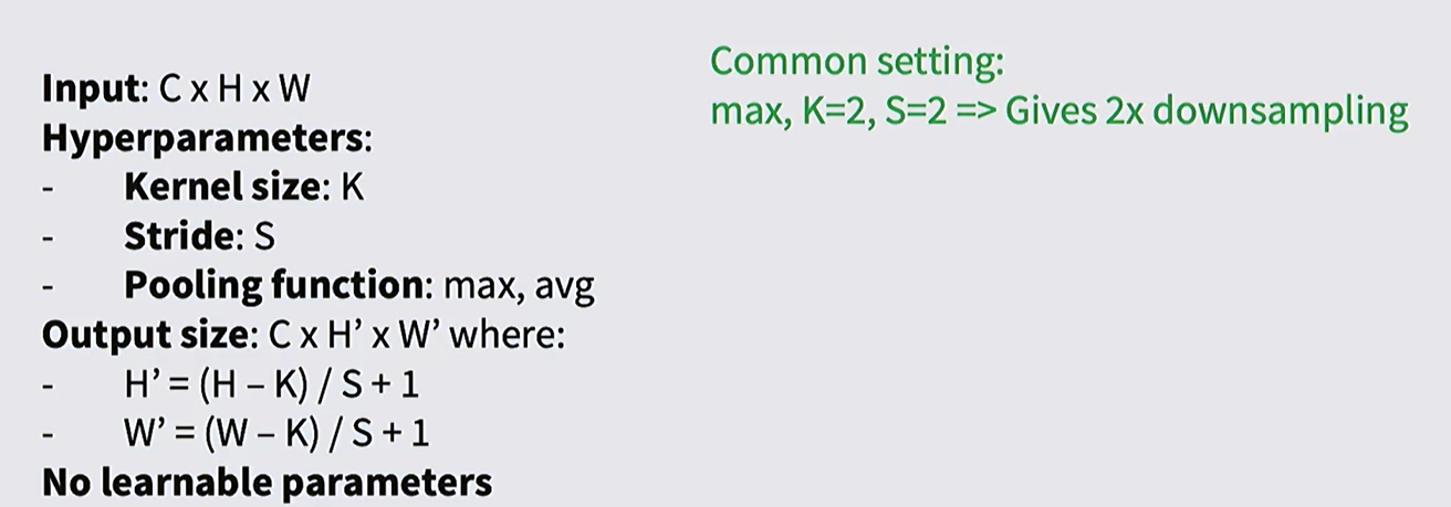
Pooling Layers
Pooling is a layer in a neural network that reduces the size of a feature map while keeping the most important information.
It works by summarizing small regions. This helps lower computation, reduce noise, and make the model less sensitive to small shifts in the input.
Pooling layers are usually interspersed with the convolution layers.
Common Methods:
- Max pooling: For each kernel, take the max entry. (Non-linear pooling)
- Average pooling (Linear pooling)
- Anti-aliased pooling
The Convolution and pooling is translation-equivariance. That is, if the input image shifts, the output feature map shifts in the same way. Applying convolution or pooling after translating the image give the sample result.
Features of images don’t depend on their locations in the image. CNNs are better at dealing with features appearing in different positions, than fully connected networks
Glossary
- affinity n. 亲和力,亲和性
- traverse
- manifold
- topical
- blob
- turn the crank on 扭动曲柄,表示执行某个系统
- facet
- spoiler alert 剧透警告
- deprecate v. 反对;抨击
- the notion of …的概念,观念
- histogram 直方图
- discretize v. 离散化
- pitch v. 扔,抛,掷
- orthogonal adj. 正交的;直角的
- convolution n. 卷积
- fencepost math 端点与间隔计数问题,植树问题
- intersperse v. 散布,散置
- prototypical adj. 原型的;典型的