Backprop is the process that lets NN learn from their own mistakes, but in a more organized fashion, and more mathematical.
Neural Networks
Linear score function: $f = Wx$, where $W \in \mathbb R^{C \times D},, x \in \mathbb R^{D}$, $D$ is for data, $C$ is for classes.
2-layer Neural Network: $f = W_2 \max(0, W_1x)$, where $W_1 \in \mathbb R^{H \times D},, x \in \mathbb R^{D}, W_2 \in \mathbb R^{C \times H}$, $D$ is for data, $C$ is for classes, $H$ is for hidden layer.
- the $\max$ function is to create a non-linearity between the two linear transformations. We call it activation function.
- In practice, we usually add a bias vector at each layer.
- 3-layer: stack the layers similarly $f = W_3\max(0,W_2 \max(0, W_1x))$.
The hidden layer can create templates for parts of the object.
Activation function: the function in the network that creates non-linearity.
- if we exclude it from the network, then the network will be degenerated into simple linear classifier.
- ReLU: $f(x) = \max(0, x)$.
- is the most popular function used in NN.
- problem: create dead neurons when the input is negative.
- has a lot of variations.
- Leaky ReLU: $f(x) = \max(0.1x, x)$
- ELU: $f(x) = \begin{cases} x,&x \ge 0 \ \alpha(e^x - 1),& x< 0 \end{cases}$
- GELU: $f(x) = x · \Phi(x)$
- SiLU: $f(x) = x · \sigma(x)$
- Sigmoid: $\displaystyle \sigma(x) = \frac{1}{1 + e^{-x}}$
- Tanh: $\displaystyle \tanh(x) = \frac{e^x - e^{-x}}{e^x + e^{-x}}$
- The choice of the activation function is mostly empirical.
Features of Neuron Network:
- more hidden neurons mean more capacity for complex functions.
- we should use explicit regularization (add a $\lambda R(W)$ in the end) to avoid overfitting the training dataset, rather than shrinking the size of neural network.
- The size of neural network implies the comprehensive ability. The choice of the size is empirical and based on given problem. Experiments are necessary.
- The ratio of regularization implies how well we want our network to be general.
biological inspirations:
- multiple input: cell body aggregates the impulses from the dendrite
- output: impulses are carried away from the cell body through the axon
Backpropagation
Computational Graph: a graph that puts together all the calculations in the neuron network.
- derivative of each node (single calculation step) is obvious.
- Based on the chain rule. the gradient of each parameter is the multiplication of its “upstream gradients”.
- This way of calculation avoid complicated calculation by human.
- computational graph representation may not be unique.
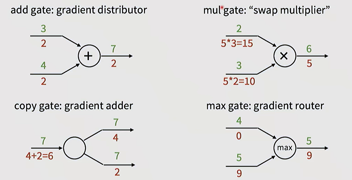
Typical patterns in gradient flow:
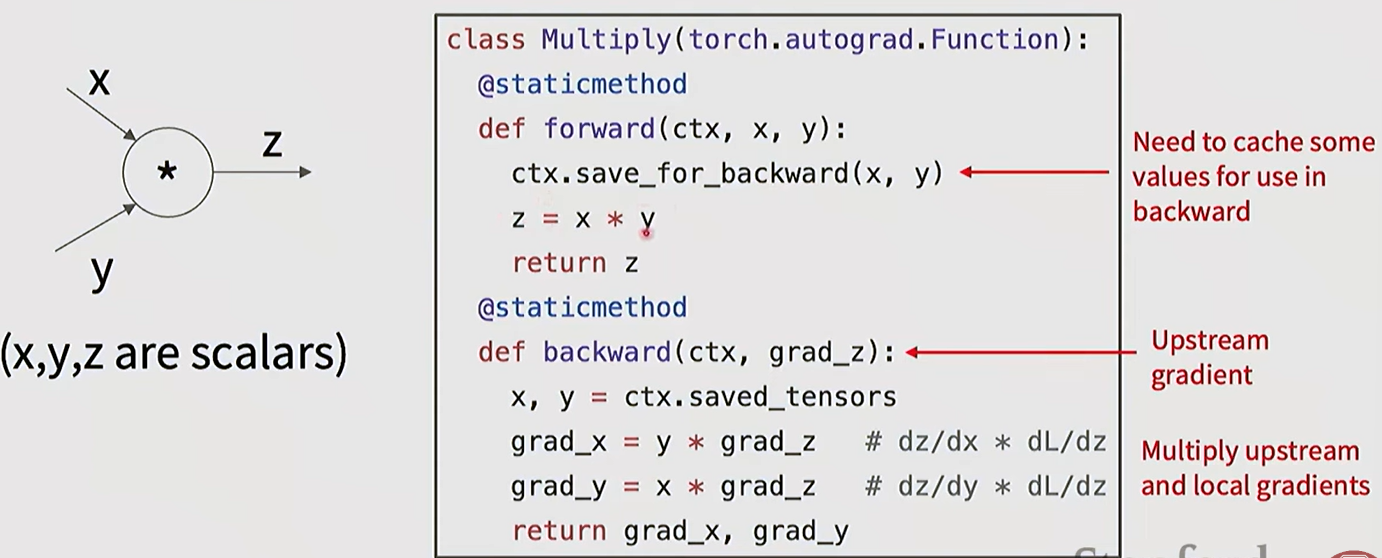
The forward / backward API can be implemented in the class function:
Backdrop with vectors/matrices:
- vector to scalar derivative: $\displaystyle \left(\frac{\partial y}{\partial x}\right)_n = \frac{\partial y}{\partial x_n}$. The derivative is a vector.
- vector to vector derivative: $\displaystyle \left(\frac{\partial y}{\partial x}\right)_{nm} = \frac{\partial y_m}{\partial x_n}$. The derivative is a Jacobian matrix.
- when doing backdrop, derivative of each node is Jacobian matrices. The multiplication become matrix-matrix or matrix-vector.
- For elementwise function, the Jacobian matrix is only diagonal and very sparse, like $\max$ function. In this case we don’t really store the matrix but calculated in backward pass function.
- matrix to scalar derivative: $\displaystyle \left(\frac{\partial y}{\partial x}\right)_{nm} = \frac{\partial y}{\partial x_{nm}}$. The size is the same as the matrix.
- matrix to matrix derivative: $\displaystyle \left(\frac{\partial y}{\partial x}\right)_{nmab} = \frac{\partial y_{ab}}{\partial x_{nm}}$. The size is the multiplication of the both matrixes.
- In general, we don’t store the Jacobian matrix because it takes a huge memory. We usually write the backward pass function to calculate the elements.
- For matrix multiply $Y = XW$ node in the loss function, the gradient is a swap: $\displaystyle \frac{\partial L}{\partial X} = \frac{\partial L}{\partial Y} W^{T},\ \frac{\partial L}{\partial W} = X^T\frac{\partial L}{\partial Y}$.
Glossary
- reiterate v. 重申
- for the sake of
- dimensionality
- terminology
- pivotal
- lump together
- rectified
- binarize 二值化
- in a nutshell 概括地说
- prescription
- metaparameter
- aggregate v. 集合,聚集
- dendrite n. 树突
- axon n. 轴突
- the ground truth
- intractable
- infeasible
- madularize
- with respect to