Regularization
We add “regularization” in the loss function, to make the system work better on test data and worse on training data.
- in other words, to avoid overfitting the data
- $\lambda$ is also a hyperparameter, to adjust the ratio of regularization.
- Bigger $\lambda$ means more contributions that regularizer has to the loss function, more constrictions to the parameters $W$, more generic boundaries and less overfitting the data.
- We should adjust the hyperparameter $\lambda$ to strike the compromise between the loss and the weights.
$$L(W) = \underbrace{\frac{1}{N}\sum_{i = 1}^N L(f(x_i,W),y_i)}_{\text{data loss}} + \underbrace{\lambda R(W)}_{\text{regularization}}$$
Examples of regularization:
- L2: $\displaystyle R(W) = \sum_k\sum_l W_{kl}^2$ allows for very small values but nonzero in some dims, and “spread out” weights among dims.
- L1: $\displaystyle R(W) = \sum_k\sum_l |W_{kl}|$ prefer pushing values into complete zero in some dims, and “sparse” weights among dims.
Ideas of regularization:
- express preference over weights
- make the model simpler on training data
- improve the optimization process
Optimization
analogy: trying to find the lowest area in the landscape, but blind-folded.
Strategy #1: Random Select Points and calc the min.
Strategy #2: Follow and move down the slope.
- the gradient is the negative vector of partial derivatives along each dim
- numeric gradient is slow and will produce resolute errors.
- analytic gradient is just a func of $W$ and is exact, fast and error-prone in implementation, where we should double-check the calc process (gradient check).
- stop sign: perform predetermined iterations, or stop when the loss is no longer significant (less than the tolerance).
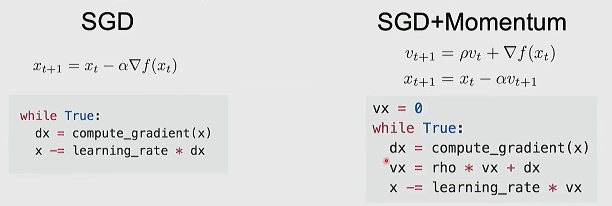
Stochastic Gradient Descent (SGD)
gradient of the loss function: $$\nabla_WL(W) = \frac{1}{N} \sum_{i = 1}^N \nabla_W L_i(x_i, y_i, W) + \lambda \nabla_W R(W)$$ if we calc the exact gradient, we have to sum up all $N$ terms, which is really time-consuming.
Idea of SGD: samples the random minibatch of dataset and do the sum each time we do the gradient descent.
- epoch: an amount of iterations to make sure all the samples in the data have been selected once.
Problems of GD/SGD:
- overshoot: learning rate is too large. Move too boldly that ends up away from the objective or jittering too wildly.
- errors: loss function has high condition number.
- local minimum: the loss function has a local minima or saddle point, where the gradient is $0$ and gets stuck. Specially, saddle point is more common in high-dim space.
- noisy: mini-batching could bring some noisy directions. (but could benefit while trying to get out from the local minimum or saddle point)
SGD + Momentum: Merge the past velocity and current gradient. This trick can solve the previous problems to some extent.
- still keep moving at local minima or saddle point
- mix the previous directions into a overall orientation, which keep roughly moving towards objective consistently.
- might help with not converging (become harder to change direction), but finding a better minimum point. (empirically)
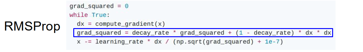
RMSProp
year proposed: 2012
Instead of saving the previous velocity, RMSProp add element-wise scaling of the gradient based on previous sum of sqr in each dim.
- step farther in dimensions which the gradient is small and closer in dimensions which the gradient is large.
- Movement is more stable because we mix the previous velocity together.
$$s_t = \rho s_{t - 1} + (1 - \rho) g_t^2$$ $$x_t = x_{t - 1} - \eta \frac{g_t}{\sqrt{s_t} + \epsilon}$$
Adam
year proposed: 2015
Adam / AdamW optimizer is the most popular optimizer in DL.
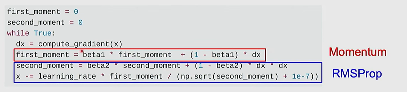
Adam mixed the idea of momentum and RMSProp.
- mix the previous velocity and current gradient.
- add element-wise scaling in each dimension based on previous sum of square gradient.
The hyperparameters beta1, beta2 are set very close to $1$ eg $0.9, 0.99$. For the first time move, the denominator is very close to $0$, which create the very large initial step. Therefore actually, we add bias correction to the two momentums.
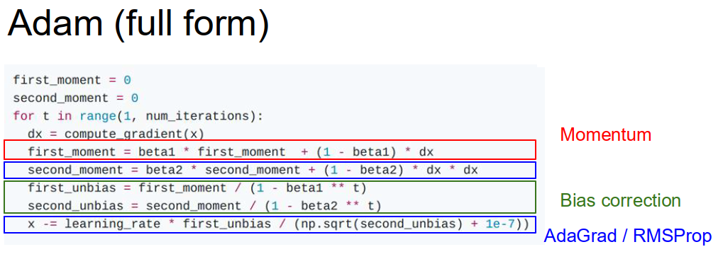
Recommended hyperparameter setting: beta1 = 0.9, beta2 = 0.999, learning_rate = 1e-3 or 5e-4.
AdamW
If the loss function includes L2 optimization, it might interfere with the Adam optimizer because we calculate the momentums on “regulated” gradient.
So we put the L2 optimization independently in the last step.
$$L’(\theta) = L(\theta_t) + \frac{\lambda}{2} \lVert \theta_t \rVert^2$$ $$g_t = \nabla_{\theta} L(\theta_t)$$ $$\theta_{t+1} = \theta_t - \alpha \left(\frac{m_t}{\sqrt{s_t} + \epsilon} + \underbrace{\lambda \theta_t}_{\text{weigh decay}}\right)$$
Learning Rate
Ideal learning rate will have a decreasing loss gradient curve.
learning rate is recommend to decay overtime.
- multiply LR by $0.1$ after epochs 30, 60, 90, etc.
- cosine LR decay: $\displaystyle \alpha_t = \frac{1}{2} \alpha_0\left(1 + \cos \frac{t\pi}{T}\right)$
- Linear LR decay: $\displaystyle \alpha_t = \alpha_0\left(1 - \frac{t}{T}\right)$
- Inverse sqrt LR decay: $\displaystyle \alpha_t = \frac{\alpha_0}{\sqrt t}$
High initial learning rate can make loss explode. We can set linearly increasing learning rate in the very beginning iterations of the training.
- Empirical rule of thumb: If you increase the batch size by $N$, also scale the initial learning rate by $N$.
Second Order Optimization
In second-order optimization, we use gradient and hessian to form quadratic approximation. And step to the minima of the approximation.
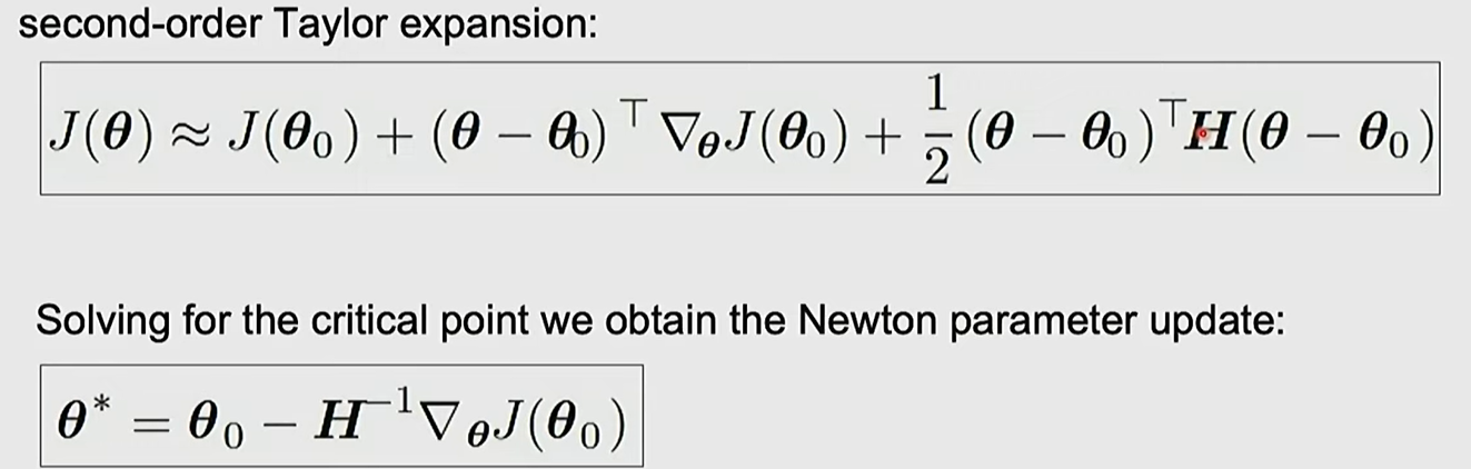
We have to calculate the hessian matrix, which mixes all the derivative parameter in pairs and brings $O(N^2)$ complexity of calculation. And calculating inverse matrix takes $O(N^3)$ time. So we don’t use 2-order optimization in large scale data generally.
Glossary
- hone in on the idea
- deformable
- intensity
- formalize v. 使形式化
- exponentiate
- rigorous
- vanilla
- level set
- traverse
- oscillate
- jitter
- empirically
- saddle
- prerequisite
- in the interest of
- rule of thumb