Generative Adversarial Networks (GANs)

High-level idea: give up on explicitly computing $p(x)$, but directly learn how to sample from a distribution that matches the training data.

We start from a simple prior $z \sim p(z)$, usually a unit Gaussian.
A generator $G$ maps $z$ to a fake sample $x = G(z)$, which induces a generator distribution $p_G$.
The goal is to make $p_G$ as close as possible to the true data distribution $p_{data}$.

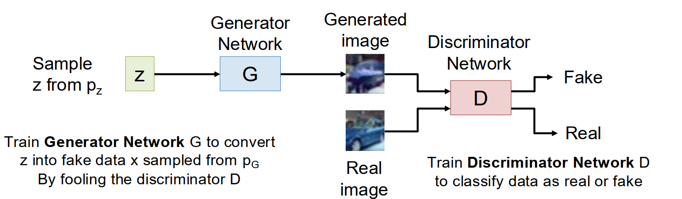
The core trick is to introduce another network, the discriminator $D$.
$D(x)$ is trained to output the probability that $x$ is real:

• $D(x) \approx 1$: looks like real data
• $D(x) \approx 0$: looks fake

So the two networks play a game:

• $D$ tries to distinguish real data from generated data.
• $G$ tries to fool $D$.

The original GAN objective is

$$ \min_G \max_D ; \mathbb E_{x \sim p_{data}} [\log D(x)] + \mathbb E_{z \sim p(z)} [\log (1 - D(G(z)))] . $$

This is a minimax game, not an ordinary single loss minimization problem. That is one major reason why GANs are hard to train: there is no single scalar training curve whose decrease clearly means “the model is getting better”.

GAN Objective

From the discriminator’s view:

• for real samples, it wants $D(x)=1$
• for fake samples, it wants $D(G(z))=0$

From the generator’s view:

• it wants the fake sample to be judged as real
• so it wants $D(G(z))=1$

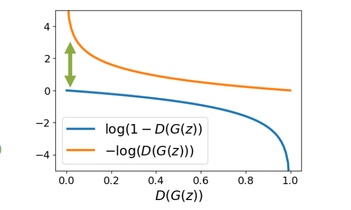
A useful practical detail is that the naive generator objective often gives very small gradients at the beginning of training.
At the start, the generator is terrible, so the discriminator can easily tell fake from real, which means $D(G(z))$ is close to $0$.
In that region, minimizing $\log(1 - D(G(z)))$ gives weak gradients for the generator.

So in practice we usually replace the generator loss with the non-saturating version:

$$ L_G = - \log D(G(z)). $$

This gives the generator much stronger gradients early in training.

GAN Architectures

In practice, both $G$ and $D$ are neural networks, historically usually CNNs.
One early important architecture was DC-GAN, which showed that GANs could work on non-toy image data.
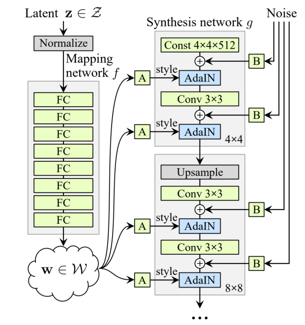
Later, StyleGAN made GAN image generation much stronger by using a more structured generator and injecting style/noise information through adaptive normalization.

For StyleGAN, a representative operation is AdaIN:

$$ \operatorname{AdaIN}(x,w,b)_i = w_i \frac{x_i - \mu(x)}{\sigma(x)} + b_i. $$

The main intuition is that style information can modulate intermediate activations layer by layer, which makes the latent space more controllable and often improves image quality.

Latent Space Interpolation

One nice property of GANs is that the latent space is often smooth.
If we sample two latent vectors $z_0$ and $z_1$, then interpolate between them,

$$ z_t = t z_0 + (1-t) z_1, \qquad x_t = G(z_t), $$

the generated images often change smoothly as $t$ varies.
This suggests that the generator has learned some meaningful structure in latent space rather than memorizing isolated points.

The understanding of GANs

GANs were very influential because they can generate extremely sharp images and have a conceptually elegant setup: one network generates, one network critiques.

But they also have obvious weaknesses:

• training is unstable
• there is no reliable loss curve to interpret
• optimization is a game
• scaling them to very large models and datasets is difficult

So GANs were dominant for several years, but later were largely displaced by diffusion models in mainstream large-scale generation.

Diffusion Models

High-level idea: instead of generating a sample in one shot, start from pure noise and repeatedly denoise it.

The basic picture is:

1. choose a simple noise distribution, usually Gaussian
2. corrupt data with different noise levels
3. train a neural network to remove a little bit of noise
4. at sampling time, start from full noise and apply the network many times

Compared with GANs, diffusion models have a much nicer training story:

• the training loss is usually an ordinary regression loss
• training is much more stable
• scaling to large datasets and large models works better in practice

The main disadvantage is that inference is slow, because generation requires many denoising steps.

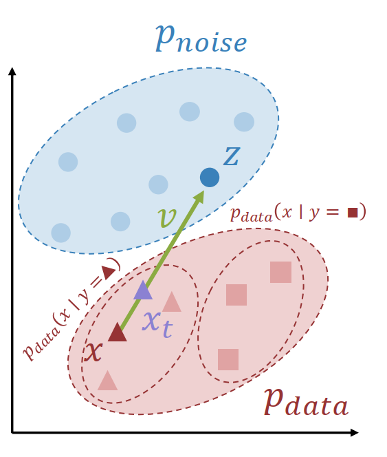
Rectified Flow

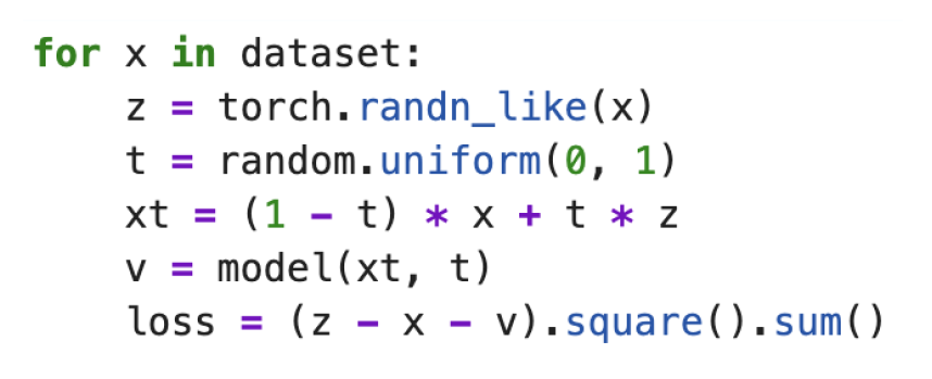
Suppose we have

• $x \sim p_{data}$
• $z \sim p_{noise}$
• $t \sim \operatorname{Uniform}(0,1)$

Then define

$$ x_t = (1-t)x + tz, \qquad v = z - x. $$

So $x_t$ is a noisy point on the straight line between data and noise, and $v$ is the velocity vector pointing from data to noise.

The network is trained to predict this velocity:

$$ L = | f_\theta(x_t, t) - v |_2^2. $$

This is surprisingly simple.
The model sees a partially noised sample $x_t$ together with the noise level $t$, and tries to predict the direction that connects data and noise.

Rectified Flow: Sampling

At inference time, we do the reverse procedure:

• sample $x_1 \sim p_{noise}$
• march from $t=1$ to $t=0$
• repeatedly predict a velocity and take a small step

A simple sampling loop is

$$ x \leftarrow x - \frac{1}{T} f_\theta(x_t, t) $$

for a sequence of timesteps from $1$ down to $0$.

So generation is an iterative transport process: move a noise sample little by little toward the data manifold.

The understanding of Rectified Flow

Why is Rectified Flow attractive?

Because the core training loop is just:

• sample a real data point
• sample a Gaussian noise point
• pick a time $t$
• interpolate linearly
• predict the velocity with an MSE loss

So diffusion is not inherently complicated at the implementation level.
A lot of complexity in the literature comes from notation and mathematical formalism, not from the core code path itself.

Conditional Rectified Flow

Most useful generative models are actually conditional.
We do not only want to generate “some sample”; we want to generate a sample conditioned on user input $y$, such as text, class label, image prompt, or video prompt.

In conditional Rectified Flow, we simply feed $y$ into the model as an additional conditioning signal:

$$ v = f_\theta(x_t, y, t). $$

Then during training the dataset provides pairs $(x,y)$, and during sampling the user provides $y$.

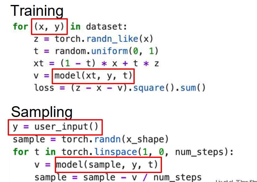
The high-level idea is unchanged: move from noise toward the data distribution.
The only difference is that now we move toward the conditional distribution $p_{data}(x \mid y)$ instead of the unconditional one.

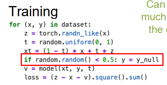
Classifier-Free Guidance (CFG)

A very important practical trick is Classifier-Free Guidance.

High-level idea: train one model to be both conditional and unconditional, then combine the two predictions at inference.

During training, we randomly drop the conditioning input $y$ with some probability.
So sometimes the model sees $(x_t, y, t)$, and sometimes it sees $(x_t, \varnothing, t)$ where the conditioning has been removed.

That means the same network can learn:

• an unconditional prediction

$$ v^\varnothing = f_\theta(x_t, y_\varnothing, t) $$

• and a conditional prediction

$$ v^y = f_\theta(x_t, y, t) $$

Then during sampling, combine them as

$$ v^{cfg} = (1+w)v^y - w v^\varnothing. $$

Here $w$ is the guidance strength.
Larger $w$ pushes the denoising direction more toward the conditional distribution, so the output follows the prompt more aggressively.

This trick is used almost everywhere in modern diffusion systems because it significantly improves conditional fidelity.
The downside is that it roughly doubles sampling cost, since the model must be evaluated twice per denoising step.

Noise Schedules

Different noise levels are not equally difficult.
At very high noise and very low noise, the optimal prediction is relatively simple; the ambiguous middle region is hardest.
So it is often suboptimal to sample $t$ uniformly during training.

A common improvement is to use a non-uniform noise schedule, often putting more weight on middle noise levels.
A popular choice is logit-normal sampling.
For very high-resolution data, practitioners often shift the schedule toward higher noise to better account for strong local pixel correlations.

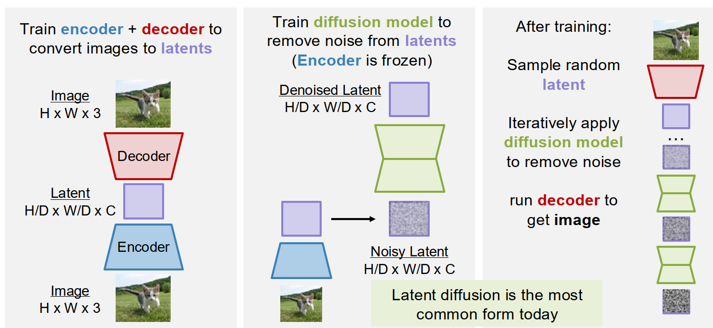
Latent Diffusion Models (LDMs)

A major practical problem is that raw-pixel diffusion is too expensive for high-resolution images.

The solution is Latent Diffusion:

1. train an encoder-decoder to map images into a compressed latent space
2. train the diffusion model in latent space instead of pixel space
3. sample a clean latent with diffusion
4. decode it back to pixels

A common setting is something like:

• image: $256 \times 256 \times 3$
• latent: $32 \times 32 \times 16$

So the diffusion model works on a much smaller representation.

This is why latent diffusion became so important: it keeps the advantages of diffusion, but makes the computation much more manageable.

How the encoder-decoder is trained

The encoder-decoder in latent diffusion is usually a VAE.
That gives us a continuous latent space that can be sampled and reconstructed.

But pure VAEs often give blurry outputs.
So modern latent diffusion pipelines add a discriminator during training of the autoencoder.
In other words, the practical system is often:

• VAE for latent compression
• GAN-style discriminator for sharper reconstructions
• diffusion model for generation in latent space

Diffusion Transformer (DiT)

Modern diffusion models often use standard Transformer blocks, leading to the Diffusion Transformer (DiT) family.

The main architectural question is no longer “can a transformer do diffusion?”
It can.
The main question is how to inject conditioning information such as timestep, text embedding, image embedding, or other controls.

Two common patterns are:

• predict scale/shift parameters from the timestep and use them to modulate activations
• use cross-attention or joint attention to inject text/image conditioning

Text-to-Image and Text-to-Video

A modern text-to-image system usually looks like this:

• text prompt $\rightarrow$ pretrained text encoder
• text embeddings + noisy latents + timestep $\rightarrow$ diffusion transformer
• clean latents $\rightarrow$ decoder $\rightarrow$ image

Text-to-video is the same idea but with an additional temporal dimension in the latent representation.
So the diffusion model now denoises a spatiotemporal latent tensor rather than a 2D latent image.

The main scaling challenge for video is sequence length.
High-resolution, high-frame-count video latents lead to extremely large token counts, so video diffusion is much more computationally demanding than image diffusion.

Diffusion Distillation

A major weakness of diffusion models is that inference is slow, since the denoising network must be run many times.

Diffusion distillation tries to reduce the number of sampling steps, sometimes even down to a single step.
The idea is to distill the behavior of a many-step diffusion process into a faster student process.

This is important because diffusion models usually beat GANs in stability and scalability, but GANs are much faster at inference.
Distillation tries to recover some of that lost speed.

Generalized Diffusion

Rectified Flow is only one special case in a broader family.

A generic training template is:

$$ x_t = a(t)x + b(t)z, $$

$$ y_{gt} = c(t)x + d(t)z, $$

$$ L = | f_\theta(x_t, t) - y_{gt} |_2^2. $$

Different diffusion formalisms correspond to different choices of these functions:

• Rectified Flow
• Variance Preserving (VP)
• Variance Exploding (VE)

Also, the training target can be chosen differently:

• x-prediction
• $\epsilon$-prediction
• v-prediction

So many apparently different diffusion papers are really different coordinate systems or parameterizations of a related underlying idea.

Other perspectives on diffusion

There are several deeper interpretations of diffusion:

• as a latent variable model, optimized by a variational lower bound
• as learning the score function $\nabla_x \log p(x)$
• as approximately solving a stochastic differential equation

These are mathematically important, but for implementation and intuition, the Rectified Flow picture is often the cleanest place to start.

Autoregressive Models on Discrete Latents

The earlier problem with autoregressive image modeling was that raw pixels create very long sequences.
But if we first learn a discrete latent representation with an encoder-decoder, then an image becomes a much shorter sequence of discrete latent tokens.

Then we can:

1. train an encoder-decoder to map images to discrete latents
2. train an autoregressive model on the latent token sequence
3. sample latent tokens autoregressively
4. decode them back to an image

Glossary

• adversarial adj. 对抗的；敌对的
• discriminator n. 判别器
• generator n. 生成器
• saturating adj. 饱和的
• interpolation n. 插值；插入
• denoise v. 去噪
• timestep n. 时间步
• guidance n. 引导；导向
• distillation n. 蒸馏
• manifold n. 流形