Supervised learning uses paired data $(x, y)$ and learns a mapping from input to label. Typical examples are classification, detection, segmentation, and captioning. Unsupervised learning only has $x$ and tries to discover hidden structure in data, such as clustering, dimensionality reduction, or density estimation. A generative model belongs to this broader unsupervised / self-supervised direction because it tries to understand the data distribution itself rather than only predict a label.
The understanding of generative vs discriminative models:
A discriminative model learns $p(y \mid x)$ and asks: given this image, which label is most likely?
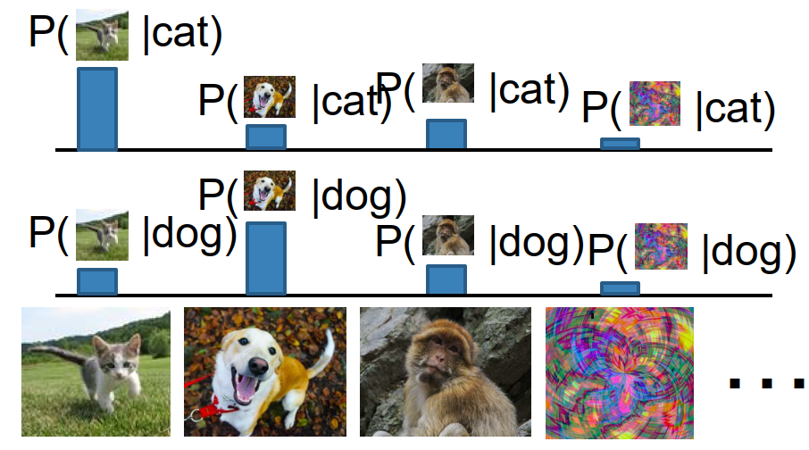
A generative model learns $p(x)$ and asks: how likely is this image itself under the data distribution?
A conditional generative model learns $p(x \mid y)$ and asks: given a condition $y$ (text, class label, another image, etc.), what outputs $x$ are plausible?
The key probabilistic difference is what competes for probability mass.
For discriminative models, for each fixed image $x$, the labels compete with each other: $$ \sum_y p(y \mid x) = 1 $$ So the model must distribute probability across labels, but different images do not compete with each other.
For generative models, all possible images compete for probability mass: $$ \int_X p(x),dx = 1 $$ This is much harder, because the model must assign low probability to unreasonable images and high probability to realistic ones. One nice consequence is that a generative model can in principle reject outliers by assigning them very small probability.
For conditional generative models, each condition $y$ induces a separate competition across all possible outputs: $$ \int_X p(x \mid y),dx = 1 $$ This is usually the most useful case in practice, since we often want controllable generation: text-to-image, language modeling, image-to-video, and so on. Even if notation sometimes writes only $p(x)$, in practice many modern systems really care about $p(x\mid y)$.
Bayes’ rule: $$ p(x \mid y) = \frac{p(y \mid x) p(x)}{p(y)} $$ So discriminative models, generative models, and conditional generative models are related, although in practice conditional models are usually trained directly instead of being assembled from the others.
Why generative models?
The main reason is ambiguity. If one input $y$ can correspond to many valid outputs $x$, then a deterministic mapping is not enough; we want a full conditional distribution: $$ p(x \mid y) $$ This is exactly what happens in language modeling, text-to-image, and image-to-video. There is not one unique correct answer; there is a space of plausible answers.
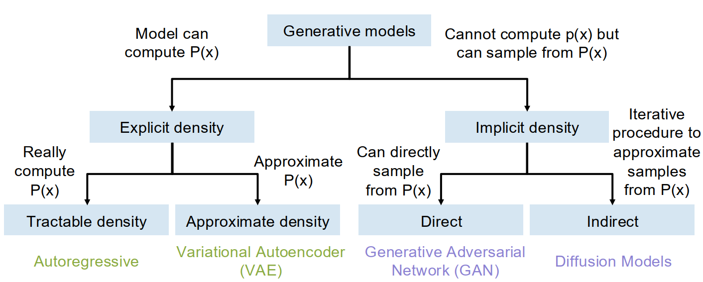
Taxonomy of generative models:
Explicit density models can compute or approximate a density value such as $p(x)$. Inside this family, autoregressive models are tractable density methods, while VAEs are approximate density methods.
Implicit density models do not directly output $p(x)$, but can sample from the data distribution. GANs are more direct samplers; diffusion models sample through an iterative procedure.
Autoregressive models
High-level idea: write down an explicit density function and train it by maximum likelihood estimation.
Suppose we have a dataset $$ x^{(1)}, x^{(2)}, \dots, x^{(N)} $$ and a neural-network density model $$ p(x) = f(x, W) $$ Then the maximum likelihood objective $$ W^* = \arg\max_W \sum_i \log p(x^{(i)}) $$ The general MLE idea is simple: choose parameters that make the training data most likely under the model.
Autoregressive factorization:
If we can view one sample as a sequence $$ x = (x_1, x_2, \dots, x_T) $$ then the chain rule of probability gives $$ p(x) = p(x_1, x_2, \dots, x_T) = \prod_{t=1}^{T} p(x_t \mid x_1, \dots, x_{t-1}) $$ So instead of modeling the full joint distribution all at once, we model one next element conditioned on the prefix. This is the basic idea of autoregressive models.
This should feel familiar: language modeling with RNNs and masked Transformers is exactly doing this. LLMs are autoregressive models over token sequences.
Autoregressive models of images:
In principle, an image can also be flattened into a sequence. One classical idea is to treat an image as a sequence of 8-bit subpixel values in scanline order, and predict each subpixel as a 256-way classification problem: $$ x_t \in {0,1,\dots,255} $$ Then an RNN or Transformer could model $$ p(x_t \mid x_1, \dots, x_{t-1}) $$ for each step.
The understanding of the limitation:
This is conceptually clean, but computationally brutal. A $1024 \times 1024$ RGB image contains about three million subpixels, so the sequence becomes far too long.
Autoregressive image modeling at raw-pixel level is too expensive, and one modern workaround is to model sequences of tiles / tokens instead of raw subpixels.
So the tradeoff is clear: autoregressive models are mathematically simple and give exact tractable density, but generation is slow and high-resolution images are expensive to model directly.
Variational autoencoders (VAEs)
High-level idea: add a probabilistic latent variable $z$ to an autoencoder, force latent codes to follow a known prior, and optimize a lower bound on log-likelihood.
Before the variational version, first recall the ordinary autoencoder.
VAE idea
A standard autoencoder has an encoder and decoder: $$ x \rightarrow z \rightarrow \hat{x} $$ It learns without labels by reconstructing the input. A common loss is L2 reconstruction: $$ \lVert \hat{x} - x \rVert_2^2 $$ After training, we can throw away the decoder and use the encoder features for downstream tasks.
But if our goal is generation, plain autoencoders have a problem: even if the decoder can map latent codes $z$ back to images, sampling a good $z$ is not easier than sampling a good $x$. The latent space learned by an ordinary autoencoder may be messy and not follow any simple distribution.
Generative process
In a VAE, we assume each data point $x$ is generated from an unobserved latent variable $z$.
We choose a simple prior, usually $$ p(z) = \mathcal{N}(0, I) $$ and a decoder distribution $$ p_\theta(x \mid z) $$ Then after training, sampling is easy:
- sample $z \sim \mathcal{N}(0, I)$
- decode through $p_\theta(x \mid z)$
The latent variable is supposed to capture hidden factors of variation such as pose, appearance, orientation, style, and so on.
Why exact likelihood is hard
If we want to train by maximum likelihood, then since $z$ is unobserved we must marginalize it out: $$ p_\theta(x) = \int p_\theta(x, z),dz = \int p_\theta(x \mid z) p(z),dz $$ The prior $p(z)$ is simple, and the decoder gives $p_\theta(x \mid z)$, but the integral over all latent variables is intractable.
Trying Bayes’ rule also leads to trouble: $$ p_\theta(x) = \frac{p_\theta(x \mid z) p(z)}{p_\theta(z \mid x)} $$ Now the hard term becomes the true posterior $$ p_\theta(z \mid x) $$ which we also cannot compute.
Variational approximation
The VAE trick is to introduce another neural network, $$ q_\phi(z \mid x) \approx p_\theta(z \mid x) $$ called the encoder or inference network. So the two networks are:
- decoder $p_\theta(x\mid z)$: latent code $z \to$ distribution over data $x$
- encoder $q_\phi(z\mid x)$: data $x \to$ distribution over latent code $z$
In practice, both are often Gaussian outputs: $$ p_\theta(x \mid z) = \mathcal{N}(\mu_{x\mid z}, \sigma^2 I) $$ $$ q_\phi(z \mid x) = \mathcal{N}(\mu_{z\mid x}, \Sigma_{z\mid x}) $$ where the encoder predicts mean and diagonal covariance of $z$, and the decoder predicts the mean of $x$. Because the decoder output is Gaussian, maximizing its log-likelihood is equivalent to minimizing an L2 reconstruction term.
ELBO
Starting from $$ \log p_\theta(x) $$ and multiplying / dividing by $q_\phi(z\mid x)$, $$ \log p_\theta(x) = \mathbb{E}{z \sim q\phi(z\mid x)} [\log p_\theta(x\mid z)]
- D_{KL}(q_\phi(z\mid x),|,p(z))
- D_{KL}(q_\phi(z\mid x),|,p_\theta(z\mid x)) $$ The last KL term is always nonnegative, so dropping it gives a lower bound: $$ \log p_\theta(x) \ge \mathbb{E}{z \sim q\phi(z\mid x)} [\log p_\theta(x\mid z)]
- D_{KL}(q_\phi(z\mid x),|,p(z)) $$ This lower bound is the ELBO (Evidence Lower Bound), and it becomes the training objective of the VAE.
The understanding of the two ELBO terms:
The first term $$ \mathbb{E}{z \sim q\phi(z\mid x)} [\log p_\theta(x\mid z)] $$ is the reconstruction term. It says: encode $x$ into a latent distribution, sample $z$, and the decoder should be able to reconstruct $x$.
The second term $$ D_{KL}(q_\phi(z\mid x),|,p(z)) $$ is the prior-matching term. It says: the encoder output should stay close to the simple prior, usually a unit Gaussian.
These two terms fight each other.
- Reconstruction wants the encoder to make each $x$ map to a very specific, almost deterministic latent code, so the decoder can reconstruct perfectly.
- Prior matching wants all encoded latents to look like one shared Gaussian cloud.
A VAE lives in the compromise between those two pressures.
Training and sampling
Training procedure:
First run input $x$ through the encoder to get $$ q_\phi(z\mid x) = \mathcal{N}(\mu_{z\mid x}, \Sigma_{z\mid x}) $$ Then apply the KL prior loss that encourages this distribution to stay near $$ \mathcal{N}(0, I) $$ Next, sample latent code $z$ using the reparameterization trick: $$ \epsilon \sim \mathcal{N}(0, I), \qquad z = \mu_{z\mid x} + \epsilon \odot \Sigma_{z\mid x} $$ Then run $z$ through the decoder to get the predicted mean of $x$, and apply reconstruction loss. Jointly maximize the ELBO.
Sampling procedure:
After training, the encoder is not needed for generation. Just sample $$ z \sim \mathcal{N}(0, I) $$ and pass it through the decoder to get a new image.
Disentangling intuition: Because the prior on $z$ is diagonal Gaussian, different dimensions are encouraged to be statistically independent. In practice, changing one coordinate of $z$ while holding others fixed can sometimes smoothly vary one interpretable factor, such as style, orientation, or thickness.
Glossary
- apportion v. 分配,分摊
- autoregressive adj. 自回归的
- intractable adj. 无法精确求解的
- latent adj. 潜在的,隐变量的
- posterior n. 后验分布
- reparameterization n. 重参数化
- disentangle v. 解耦,分离