Self-Supervised Learning
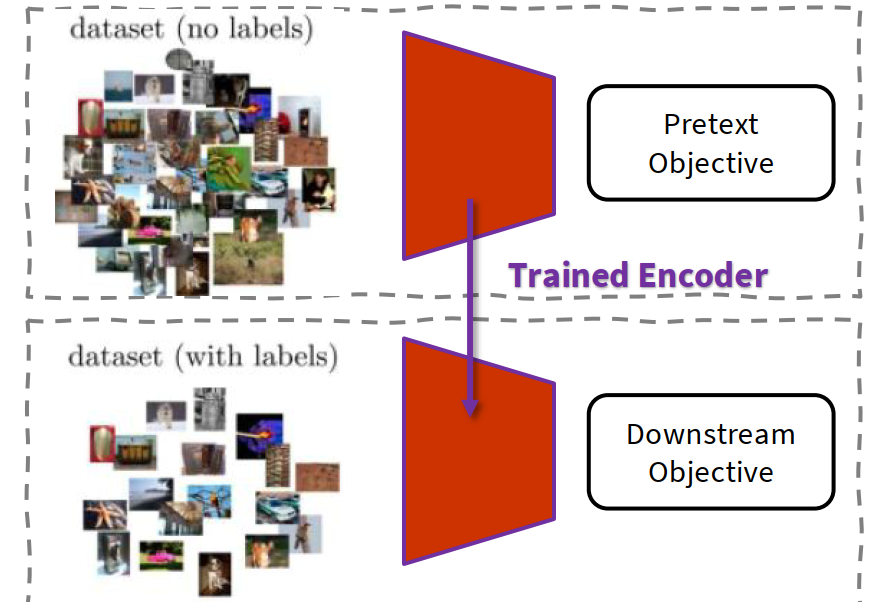
High-level idea: We want to learn a strong encoder from a large amount of unlabeled data by defining a task whose supervision is automatically generated from the data itself. After that, we transfer the learned encoder to a downstream supervised task.
A neural network often learns useful representations / features / embeddings / latent space before the final classifier layer. If those representations are already good, then a shallow classifier can often solve the downstream task well.
The main bottleneck of large-scale supervised learning is not only model size or compute, but also the need for a large amount of manual labels.
The understanding of self-supervised learning:
- The point is not to remove supervision completely; the point is to replace manual annotation with supervision that is generated from the raw data.
- So it is called self-supervised: the data itself provides the targets.
- We first solve a pretext task, then transfer the encoder to a downstream task.
Pretext task:
- defined directly from the raw data;
- does not require manual annotation;
- can still be trained with standard supervised objectives such as classification or regression.
Downstream task:
- the actual application we care about;
- usually has fewer labeled samples;
- uses the pretrained encoder as a feature extractor or as an initialization.
generic framework:
- encoder $f(\cdot)$ maps the input to a learned representation;
- another module (decoder / classifier / regressor) predicts automatically generated targets;
- after pretraining, we keep the encoder and train a small head for the target task.
How to evaluate a self-supervised method:
- pretext task performance itself;
- representation quality (for example linear evaluation);
- robustness and transferability;
- the most important one: downstream task performance.
common protocol:
- pretrain an encoder on lots of unlabeled data;
- freeze or partially freeze the encoder;
- train a linear layer or a small head on labeled downstream data.
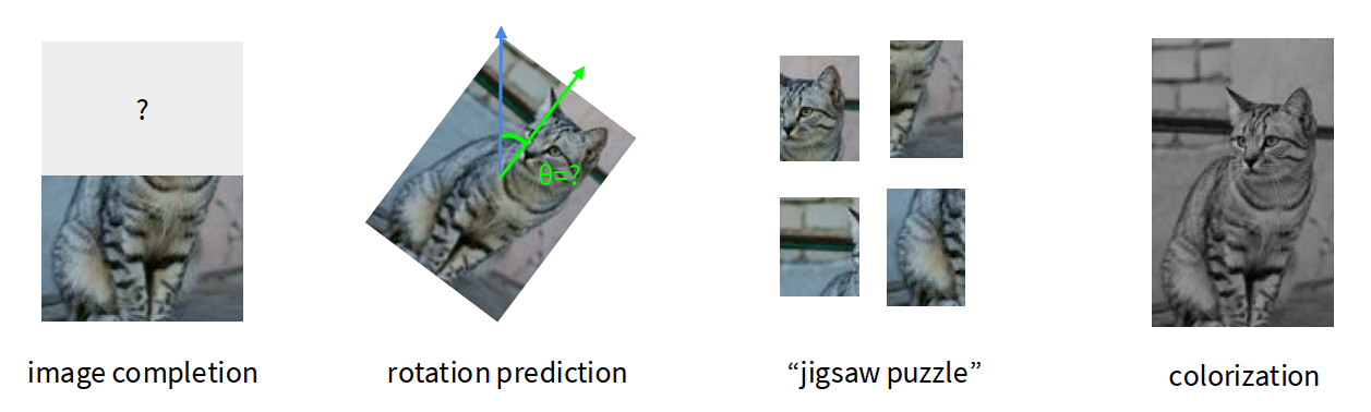
Pretext tasks from image transformations
High-level idea: We corrupt, transform, or partially hide the image, then ask the network to recover some property of the original image. To solve such tasks, the model is forced to learn meaningful visual structure.
The understanding of pretext tasks:
- A good pretext task should require some form of visual common sense.
- It should not rely only on trivial local statistics.
- We usually do not care about the pretext task itself; we care about whether the learned features help classification, detection, or segmentation later.
Rotation prediction:
- Rotate the image by one of ${0^\circ, 90^\circ, 180^\circ, 270^\circ}$.
- Train the network to predict which rotation was applied.
- This is a 4-way classification problem.
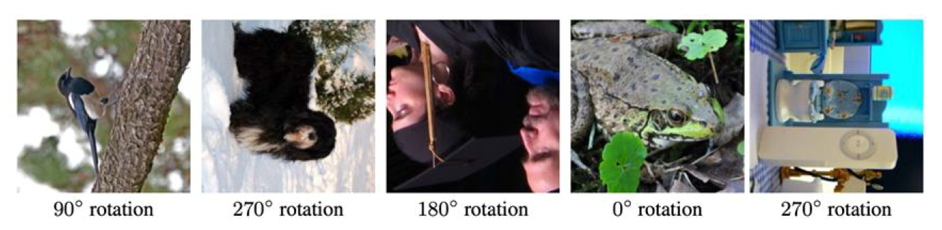
The intuition is that a model can recognize the correct rotation only if it understands what the object should look like in its normal orientation.
A useful way to think:
- if the model knows that a bird or a face is upside down, then it has already learned some semantic structure;
- therefore the intermediate representation may be transferable.
Empirically, rotation prediction gives much better downstream performance than random initialization, and on some tasks it can get surprisingly close to full supervised pretraining.
Another interesting observation is that self-supervised attention maps are often more holistic than those from a purely supervised classifier. A supervised model may focus only on the minimum discriminative region, while a self-supervised model often needs broader understanding of the image.
Relative patch location / jigsaw puzzle:
- Split the image into patches, for example a $3 \times 3$ grid.
- Either predict the relative location of one patch with respect to another, or predict the correct permutation from a set of candidate permutations.
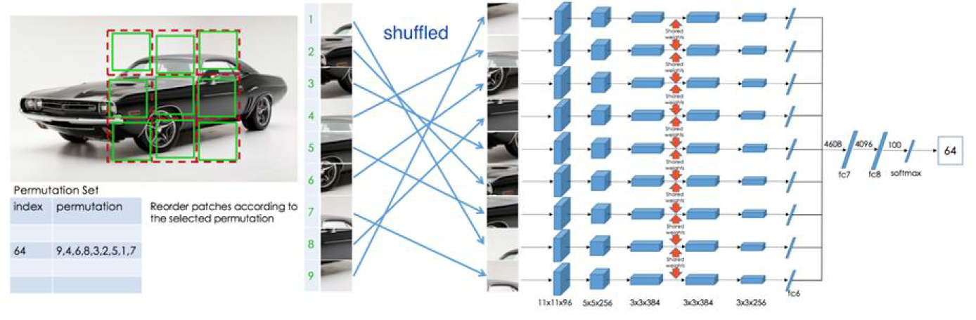
This forces the model to learn:
- object part relations;
- rough spatial layout;
- some notion of global structure instead of isolated texture.
However, this kind of task can still become somewhat tied to a specific handcrafted objective. It may learn spatial reasoning, but not necessarily the most general representation.
Inpainting / image completion:
- Mask a region of the image.
- Train the model to reconstruct the missing pixels.
- This is an autoencoder-like setup.
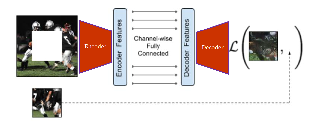
If the masked region is large enough, the model must infer semantics and context instead of only copying nearby pixels.
A simple reconstruction objective can be written as:
$$ \mathcal L_{\text{recon}} = | M \odot (x - \hat x) |^2 $$
where $M$ is the mask and the loss is only computed on masked pixels.
One issue is that pixel-space reconstruction often encourages blurry averages. Because many plausible completions exist, minimizing MSE tends to predict something smooth. This is why adversarial losses were later added in some inpainting work, though the main self-supervised idea is already visible in the reconstruction setup itself.
Colorization:
- Input the grayscale or luminance channel.
- Predict the missing color channels.
This is another pretext task that needs semantic understanding, because realistic colors often depend on object identity and context.
A related idea is the split-brain autoencoder:
- split the image channels into two groups;
- predict one group from the other, and vice versa;
- concatenate learned features from both streams.
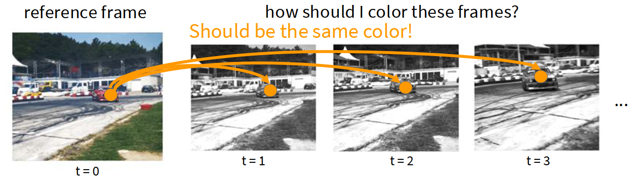
For videos, colorization becomes even more interesting. If one frame has the correct color and later frames are gray, then predicting future colors encourages the model to learn correspondences over time. In other words, tracking can emerge from color propagation.
Masked Autoencoders (MAE)
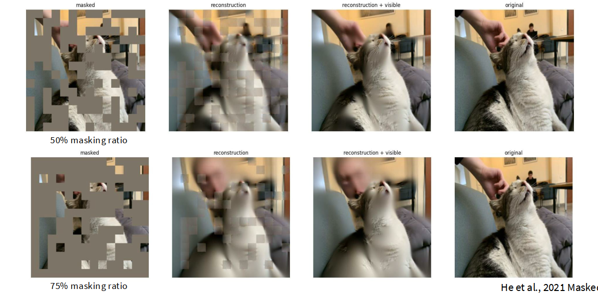
High-level idea: Instead of designing many handcrafted pretext tasks, we can use a more general reconstruction task: mask a very large portion of the image and reconstruct it.
MAE became very influential because it is simple, scalable, and works especially well with Vision Transformers.
core design:
- split the image into non-overlapping patches;
- randomly mask a large portion, often around $75%$;
- feed only the visible patches into the encoder;
- let a lightweight decoder reconstruct the full image.
MAE encoder:
- only processes visible patches;
- uses linear patch embedding + positional embedding;
- then standard transformer blocks;
- because it only sees a small subset of patches, the encoder can be made very large.
MAE decoder:
- receives encoder outputs;
- inserts shared mask tokens at missing locations;
- adds positional embeddings again;
- uses transformer blocks to reconstruct pixels.
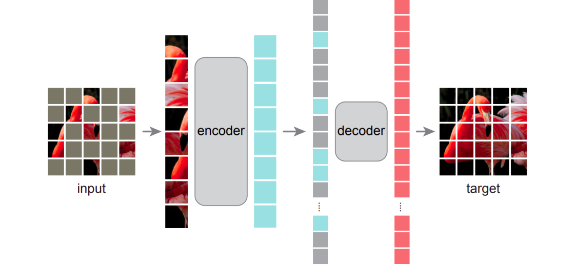
This is an asymmetric autoencoder:
- encoder is the important part for downstream use;
- decoder only serves reconstruction during pretraining;
- decoder can therefore be lightweight and flexible.
The loss is usually pixel-space MSE:
$$ \mathcal L_{\text{MAE}} = \frac{1}{|\mathcal M|} \sum_{i \in \mathcal M} | x_i - \hat x_i |^2 $$
where $\mathcal M$ is the set of masked patches.
Why high masking ratio helps:
- if masking is too weak, reconstruction becomes too easy;
- if masking is aggressive, the model must infer global structure;
- the encoder is also cheaper because it processes only the visible fraction.
So MAE is not just masking for the sake of masking. The masking ratio controls how hard and how meaningful the task is.
Linear probing vs full fine-tuning:
- Linear probing: freeze the pretrained encoder and only train a linear classifier. This mainly measures the quality of the learned representation.
- Fine-tuning: continue training the pretrained encoder together with the downstream head. This measures the practical usefulness of the model.
The understanding of MAE:
- It is much more general than many early hand-designed pretext tasks.
- It shifts the focus from “guess this specific transformation” to “understand enough of the scene to reconstruct what is missing”.
- This is one reason MAE became a standard pretraining strategy.
Contrastive representation learning
High-level idea: Instead of reconstructing pixels, learn a representation space where two related views are close and unrelated views are far apart.
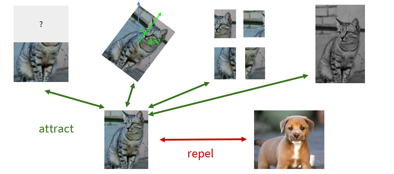
So we define:
- $x$: reference sample;
- $x^+$: positive sample, usually another view of the same instance;
- $x^-$: negative sample, usually a different instance.
We want:
- high score for $(x, x^+)$;
- low score for $(x, x^-)$.
A standard formulation is the InfoNCE loss:
$$ \mathcal L_{\text{InfoNCE}} = - \log \frac{\exp(s(f(x), f(x^+)))}{\exp(s(f(x), f(x^+))) + \sum_{i=1}^{N-1} \exp(s(f(x), f(x_i^-)))} $$
If a temperature $\tau$ is used and the score is cosine similarity, then one common choice is:
$$ s(z_i, z_j) = \frac{z_i^\top z_j}{\tau |z_i|,|z_j|} $$
The understanding of InfoNCE:
- It looks like an $N$-way softmax classification loss.
- The model is learning to find the positive sample among many candidates.
- It is also connected to maximizing mutual information between related views.
- More negative samples usually make the learning signal stronger.
SimCLR
Recipe:
- take one image;
- apply two random augmentations to get two correlated views;
- pass both through the same encoder $f(\cdot)$;
- pass features through a projection head $g(\cdot)$;
- apply InfoNCE in the projected space.
All other non-positive samples in the minibatch act as negatives.
Why a projection head helps:
- contrastive learning wants invariance to augmentation;
- enforcing this directly in the main representation can discard information useful for downstream tasks;
- the projection head lets the contrastive objective act in $z$-space, while the encoder representation $h$ can keep richer information.
This is why SimCLR usually uses:
- encoder output $h$ for downstream tasks;
- projected vector $z = g(h)$ for contrastive loss.
A major practical issue is that SimCLR usually needs a very large batch size, because batch elements provide the negative samples.
MoCo
Momentum Contrastive Learning (MoCo) solves part of the large-batch problem.
Key ideas:
- keep a running queue of negative keys;
- use a query encoder for the current batch;
- use a key encoder updated by momentum rather than direct backpropagation;
- use the queue instead of requiring all negatives to come from the current minibatch.
The momentum update is conceptually:
$$ \theta_k \leftarrow m\theta_k + (1-m)\theta_q $$
where $\theta_q$ and $\theta_k$ are parameters of the query and key encoders.
Why MoCo matters:
- it decouples minibatch size from negative sample size;
- it is much more memory efficient than huge-batch SimCLR;
- MoCo v2 combines the good parts of SimCLR (strong augmentation and nonlinear projection head) with the queue-based design.
CPC
Contrastive Predictive Coding (CPC) is a sequence-level contrastive method.
Instead of contrasting two random views of the same image instance, CPC uses context to predict the future in a sequence.
main idea:
- encode samples into latent vectors $z_t$;
- summarize past context into $c_t$ using an autoregressive model;
- contrast the true future latent $z_{t+k}$ against negatives.
So CPC is especially natural for audio, video and sequential data.
For images, one can also impose a sequence structure by turning image patches or rows into a sequence, but CPC is generally more associated with temporal or ordered data.
newer SSL methods
Later methods such as MoCo v3 and DINO / DINOv2 push self-supervised learning further, especially for Vision Transformers. A useful high-level trend is:
- early SSL often relied on handcrafted pretext tasks;
- then contrastive learning became dominant;
- newer methods increasingly use self-distillation or teacher-student style objectives and often learn stronger ViT representations.
moved from specific pretext tasks to more general representation learning objectives.
Summary
Self-supervised learning is about training an encoder without manual labels, by creating supervision from the data itself.
two major families:
- Pretext tasks from transformations / reconstruction: rotation, jigsaw, inpainting, colorization, MAE.
- Contrastive learning: SimCLR, MoCo, CPC, and later teacher-student methods.
Early pretext tasks teach the model some form of visual common sense. MAE makes reconstruction more scalable and general and contrastive learning directly shapes the representation space.
The final goal is always to learn features that transfer well to downstream tasks such as classification, detection, and segmentation.
Glossary
- pretext task n. 预文本任务;为学习表示而人为设计的自监督任务
- downstream task n. 下游任务;最终真正关心的应用任务
- latent space n. 潜在空间
- linear probing n. 线性探测;冻结主干后只训练线性分类器
- inpainting n. 图像修复;补全遮挡区域
- colorization n. 图像上色
- masking ratio n. 掩码比例
- contrastive adj. 对比式的;通过拉近正样本、推远负样本来学习
- negative sample n. 负样本
- mutual information n. 互信息
- momentum encoder n. 动量编码器
- temporal coherence n. 时间一致性