Running example: Llama3-405B
- Recently, many frontier models do not share training details.
- Llama3 is important not just because it is strong, but because its paper shares many details about the model, hardware, and training system.
- So this lecture is less about one specific model, and more about the general recipe of how modern large models are actually trained.
GPU Hardware
A GPU is a Graphics Processing Unit.
- originally designed for graphics
- now used as a general parallel processor
- modern deep learning training is basically built around exploiting this parallelism
Inside an NVIDIA H100:
- Compute cores are in the center.
- Around them there are 80 GB of HBM memory.
- Memory bandwidth from HBM to the compute cores is about 3352 GB/sec.
Memory hierarchy matters a lot.
- H100 also has 50 MB of L2 cache.
- It has 132 Streaming Multiprocessors (SMs) enabled.
- Physically there may be 144, but only 132 are enabled due to yield / binning.
The understanding of GPU hierarchy:
- deep learning is not only about neural networks; it is also heavily about computer architecture.
- larger memories are farther away and slower.
- smaller memories are closer to compute and faster.
- efficient training means trying to keep computation close to the fast part of the hierarchy as much as possible.
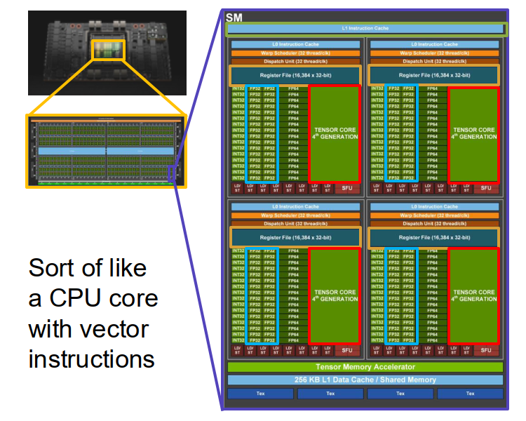
Inside one H100 SM:
- 256 KB L1 cache and 256 KB registers
- 128 FP32 cores
- 4 Tensor Cores
The FP32 cores compute scalar-style operations like $a x + b$.
- one such operation is about 2 FLOPs
- so one SM can do about 256 FLOP / cycle through FP32 cores
The Tensor Cores are more important for deep learning.
- they compute matrix-style operations like $AX + B$
- one Tensor Core operation corresponds to a small matrix multiply block
- one SM can do about 4096 FLOP / cycle through Tensor Cores
- they usually use mixed precision: low precision inputs, higher precision accumulation
The understanding of Tensor Cores:
- Tensor Cores are where most of the modern training throughput comes from.
- if your code does not hit Tensor Cores effectively, training may become much slower.
- this is why data types like FP16 / BF16 are not just implementation details; they strongly affect speed.
GPUs have become much faster.
- K40 $\to$ P100 $\to$ V100 $\to$ A100 $\to$ H100 $\to$ B200
- the big jump came when Tensor Cores became central
- roughly speaking, the lecture emphasizes a ~1000x speedup since 2013
But per-device speedup is only part of the story. We also train with many GPUs at the same time.
Cluster hierarchy:
- 1 H100 GPU: 3352 GB/sec inside the GPU
- 1 server: 8 GPUs, about 900 GB/sec between GPUs
- 1 rack: 2 servers = 16 GPUs
- 1 pod: 192 racks = 3072 GPUs, about 50 GB/sec between GPUs
- 1 cluster: 8 pods = 24,576 GPUs, with even slower cross-pod communication
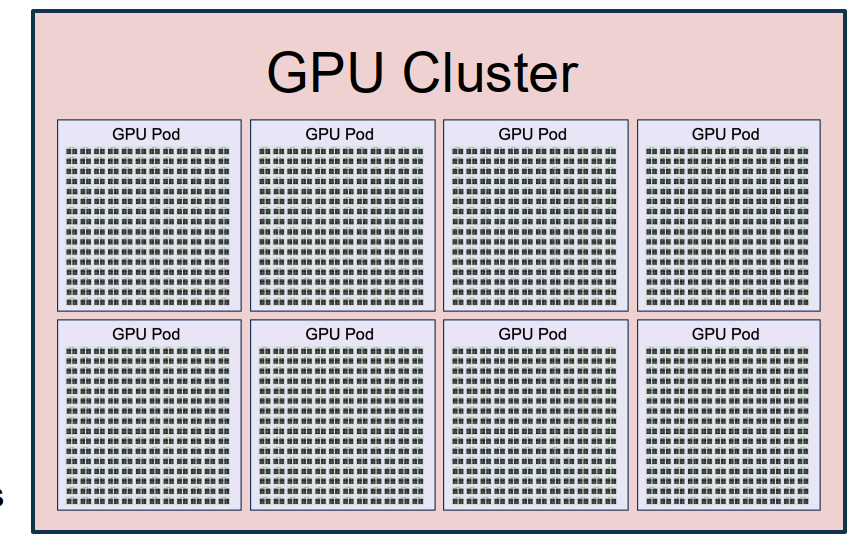 The understanding of cluster hierarchy:
 - as we move outward from one GPU to a full cluster, communication becomes slower and slower.
- so distributed algorithms should try to use fast communication locally and minimize slow global communication.
- this is the main systems reason why we need multiple kinds of parallelism.
We can think of the whole cluster as one giant computer.
- 24,576 GPUs
- 1.875 PB of GPU memory
- 415M FP32 cores
- 13M Tensor Cores
- 24.3 EFLOP/sec
The goal is to train one giant neural network on top of this giant machine.
Other training chips also exist.
- Google TPU
- AMD MI325X
- AWS Trainium2
But the lecture mainly uses NVIDIA H100 and Llama3 as the main concrete example.
Distributed Training: Basic Idea
A transformer with $L$ layers operates on tensors of shape $$ (\text{Batch}, \text{Sequence}, \text{Dim}). $$
This immediately gives multiple axes along which we can split computation:
- Data Parallelism (DP): split on Batch
- Context Parallelism (CP): split on Sequence
- Tensor Parallelism (TP): split on Dim
- Pipeline Parallelism (PP): split on Layers
This lecture’s main message is that large-scale training is basically about splitting computation along these axes while managing communication cost.
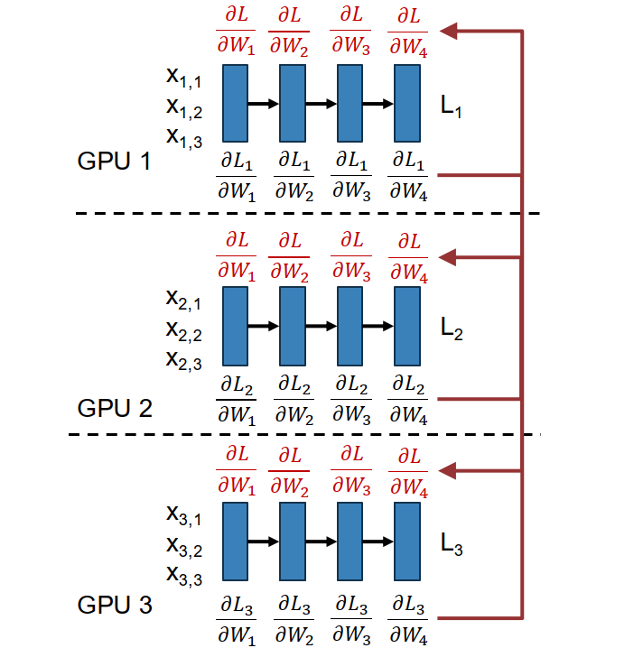
Data Parallelism and Sharding
High-level idea: use a larger effective minibatch by splitting it across many GPUs.
Suppose each GPU handles $N$ samples and we have $M$ GPUs. Then the full loss can be written as $$ L = \frac{1}{MN}\sum_{i=1}^{M}\sum_{j=1}^{N} \ell(x_{i,j}, W). $$
Because gradients are linear, $$ \frac{\partial L}{\partial W} = \frac{1}{M}\sum_{i=1}^{M} \left( \frac{1}{N}\sum_{j=1}^{N} \frac{\partial}{\partial W} \ell(x_{i,j}, W) \right). $$
So each GPU can compute its own local gradient first, and then we average them.
Steps of Data Parallelism:
- each GPU keeps its own copy of the model and optimizer
- each GPU loads a different minibatch
- each GPU runs forward to compute local loss
- each GPU runs backward to compute local gradients
- gradients are averaged across GPUs (all-reduce)
- each GPU updates its own local weights
Important point:
- step 4 and step 5 can overlap
- while lower layers are still doing backward computation, upper-layer gradients can already be communicated
- this is a typical pattern in distributed training: overlap computation and communication
Problem of naive DP: model size is limited by one GPU’s memory.
If each parameter needs:
- parameter value
- gradient
- Adam $\beta_1$
- Adam $\beta_2$
then each parameter needs about 4 numbers. If each number uses 2 bytes, then one parameter needs about 8 bytes total.
So:
- 1B params $\approx 8$ GB
- 10B params $\approx 80$ GB
That already fills up one H100. So pure DP is not enough for very large models.
Fully Sharded Data Parallelism (FSDP)
High-level idea: split model weights across GPUs instead of storing a full copy on each GPU.
Each weight block $W_i$ is owned by one GPU. That owner GPU also stores:
- its gradients
- its optimizer state
Main procedure of FSDP:
- before forward for layer $i$, the owner of $W_i$ broadcasts it to all GPUs
- all GPUs run forward on that layer
- non-owner GPUs delete their local copy of $W_i$ to save memory
- during forward of $W_i$, we can prefetch $W_{i+1}$
- before backward for layer $i$, the owner broadcasts $W_i$ again
- all GPUs run backward and compute local $\partial L / \partial W_i$
- all GPUs send their local gradients to the owner of $W_i$
- the owner updates $W_i$
The understanding of FSDP:
- we trade more communication for much lower memory usage.
- the weights are not permanently replicated on every GPU.
- they are brought in when needed, used, and then discarded.
- this lets us train models that would never fit in one device.
There is also an important optimization:
- do not delete the last weight right after forward, because backward will immediately need it again.
Another important engineering idea is overlap:
- fetch $W_i$ while computing with $W_{i+1}$
- send gradients and update $W_i$ while computing with $W_{i-1}$
So, in a good implementation, many things happen at the same time.
Hybrid Sharded Data Parallelism (HSDP)
High-level idea: combine FSDP and DP in a 2D organization of GPUs.
Suppose we split GPUs into $M$ groups of $K$ GPUs.
- inside each group of $K$ GPUs: do FSDP
- across the $M$ groups: do ordinary DP
So GPUs are organized like a 2D grid.
Inside an FSDP group, communication is heavy:
- weights in forward
- weights in backward
- gradients in backward
So communication cost is about 3x model size inside the group.
Across DP groups, we only need to communicate gradients, so it is lighter.
Therefore:
- keep the FSDP group inside fast interconnects like one node or one pod
- allow the DP communication to happen across slower interconnects
This is the first clear example where the algorithm is explicitly designed around the physical topology of the cluster.
Activation Checkpointing and MFU
Even after FSDP / HSDP, activations can still fill up memory.
For Llama3-405B:
- 126 transformer layers
- $D = 16{,}384$
- sequence length $= 4096$
Just the FFN hidden activations already take $$ 2 \cdot 126 \cdot (4 \cdot 16384) \cdot 4096 \text{ bytes} \approx 63 \text{ GB}. $$
So activations alone are already huge.
Activation Checkpointing
High-level idea: do not keep every activation in memory; recompute some of them during backward.
A layer can be viewed as two functions:
- forward: compute next-layer activations
- backward: compute previous-layer gradients
If we keep all activations normally, then:
- forward + backward cost is $O(N)$ compute
- memory is $O(N)$
If we do full recomputation, then:
- compute becomes $O(N^2)$
- memory becomes $O(1)$
That saves memory, but quadratic compute is too expensive.
So instead, save one checkpoint every $C$ layers. Then:
- compute: $O(N^2 / C)$
- memory: $O(C)$
If we choose $$ C = \sqrt{N}, $$ then we get
- compute: $O(N\sqrt{N})$
- memory: $O(\sqrt{N})$
This is the practical tradeoff.
The understanding of activation checkpointing:
- memory is often the bottleneck, not arithmetic itself.
- so it is worth doing extra compute if that extra compute lets the model fit.
- checkpointing is a classic example of trading compute for memory.
Scaling Recipe
A rough practical recipe from the lecture:
- use DP up to about 128 GPUs for models around 1B params
- always try to set per-GPU batch size large enough to make good use of memory
- if model is larger than about 1B, consider FSDP
- add activation checkpointing when activations become the memory bottleneck
- if you have more than about 256 GPUs, consider HSDP
- if you have more than about 1K GPUs, models bigger than about 50B params, or very long sequence lengths, then you likely need more advanced strategies like CP / PP / TP
This recipe is only a rough guideline, but it gives the main intuition of when each trick becomes necessary.
HFU and MFU
There are many knobs to tune in distributed training. A central idea of the lecture is: tune the system to maximize MFU.
HFU = Hardware FLOPs Utilization
- fraction of theoretical matrix multiply performance we actually achieve
- for large matrix multiply on H100, the lecture shows roughly ~80% HFU
But HFU is only about matrix multiply itself. It ignores things like:
- checkpoint recomputation
- optimizer step
- data loading
- preprocessing
- communication overhead
So HFU is not enough.
MFU = Model FLOPs Utilization
The lecture defines a practical recipe:
- compute total theoretical matrix-multiply FLOPs in forward + backward
- look up theoretical peak FLOPs/sec of the device
- compute theoretical minimum time $$ t_{\text{theoretical}} = \frac{\text{FLOP}{\text{theoretical}}}{\text{FLOP/sec}{\text{theoretical}}} $$
- measure actual iteration time $t_{\text{actual}}$
- define $$ \text{MFU} = \frac{t_{\text{theoretical}}}{t_{\text{actual}}} $$
The understanding of MFU:
- MFU asks: what fraction of the GPU’s peak capability is actually being used for useful model computation?
- it is a much better end-to-end metric for tuning a distributed training system.
The lecture’s rule of thumb:
- MFU > 30% is good
- MFU > 40% is excellent
Another subtle point:
- newer hardware can sometimes get worse MFU
- because peak FLOPs are increasing faster than memory bandwidth
- so the device becomes harder to fully feed
Other Parallelism
Context Parallelism (CP)
High-level idea: split along the sequence dimension.
This is mainly used for transformers with very long sequence length.
Some parts are easy to parallelize over sequence:
- normalization
- residual connections
MLP is also easy in structure, but weights still exist, so gradients must be synchronized much like DP.
The hardest part is the attention operator, because attention couples tokens across the whole sequence.
Two ideas mentioned in the lecture:
- Ring Attention: distribute blocks of the attention matrix across GPUs; powerful but complex
- Ulysses: parallelize over heads instead of directly distributing the full attention matrix; simpler but limited by number of heads
Llama3 example:
- Stage 1: sequence length 8192, no CP
- Stage 2: sequence length 131,072, with 16-way CP
- that means each GPU effectively handles 8192 tokens
Pipeline Parallelism (PP)
High-level idea: split the model layers across GPUs.
Each GPU owns a chunk of consecutive layers. Activations must be passed across GPU boundaries.
The naive problem is the bubble. Because of sequential dependency, many GPUs sit idle waiting for work. With $N$-way PP, the max MFU can be only $$ \frac{1}{N}. $$
That is very bad.
The main fix is to use multiple microbatches. Instead of sending one batch through the whole pipeline, run several microbatches simultaneously and let them flow through the pipeline like an assembly line.
Example from the lecture:
- 4-way PP with 4 microbatches
- max MFU increases from $$ \frac{1}{4}=25% $$ to $$ \frac{16}{28} \approx 57.1%. $$
The understanding of pipeline parallelism:
- PP saves memory by splitting layers across devices.
- but it introduces sequential dependence.
- microbatching is used to reduce idle time and shrink the bubble.
Tensor Parallelism (TP)
High-level idea: split the weight matrix of one linear layer across GPUs, so GPUs cooperate on one matrix multiply.
If $$ XW = Y, $$ then in TP we split $W$ into blocks $$ W_1, W_2, \dots, W_k $$ and each GPU computes one block result: $$ Y_i = XW_i. $$
The problem is that after forward, these parts of $Y$ normally need to be gathered. That communication is expensive.
A key trick in the lecture is for two consecutive TP layers:
- shard the first layer and second layer in complementary directions
- then each GPU can continue the next computation locally without immediately gathering all of $Y$
For example, after the first layer we get $$ Y = [Y_1, Y_2, Y_3, Y_4], $$ then the second layer can be arranged so that each GPU computes $$ Z_i = Y_i U_i, $$ and finally $$ Z = Y_1U_1 + Y_2U_2 + Y_3U_3 + Y_4U_4. $$
So communication can be postponed and reduced.
The understanding of TP:
- TP is for when a single matrix multiply is too large for one device.
- it is especially natural inside transformer MLP blocks and other large linear layers.
- the whole trick is to arrange sharding so that intermediate activations do not need to be gathered too early.
ND Parallelism
For the largest models, the answer is not choosing one method. The answer is using all of them together.
This is sometimes called ND Parallelism.
- DP on Batch
- CP on Sequence
- PP on Layers
- TP on Dim
So GPUs are organized in a higher-dimensional grid, and a GPU’s rank tells us where it lies along each parallelism dimension.
So modern large-scale training is really about composing multiple kinds of parallelism in a way that respects the cluster communication hierarchy and maximizes MFU.
Glossary
- yield / binning
- HBM (High-Bandwidth Memory)
- Tensor Core:
- throughput
- all-reduce
- prefetch: 预取
- bubble
- MFU (Model FLOPs Utilization)
- HFU (Hardware FLOPs Utilization)